Monday, December 10, 2018
Amazing Demonstration of the Digits of Pi
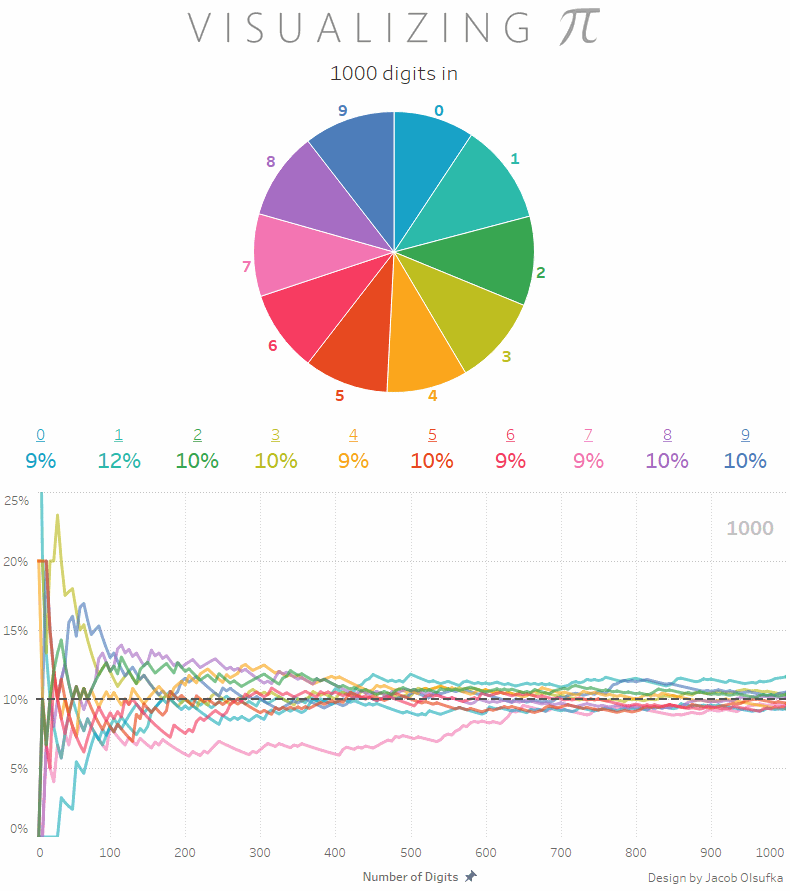
You probably know that pi made up of a series of digits that theoretically go on forever. Scientists have computers calculating the digits of pi, making it up to 2 quadrillion! Today, I found this great GIF that shows the count of digits (0 through 9) in the first 1000 digits of pi - pretty cool:
Sunday, November 25, 2018
Statistics Sunday: Introduction to Regular Expressions
In my last Statistics Sunday post, I briefly mentioned the concept of regular expressions, also known as regex (though note that in some contexts, these refer to different things - see here). A regular expression is a text string, which you ask your program to match. You can use this to look for files with a particular name or extension, or search a corpus of text for a specific word or word(s) that match a certain pattern. This concept is used in many programming languages, and R is no exception. In order to use a regular expression, you need a regular expression engine. Fortunately, R base and many R packages come with a regular expression engine, which you call up with a function. In R base, those functions are things like grep, grepl, regexpr, and so on.
Today, I want to talk about some of the syntax you use to describe different patterns of text characters, which can include letters, digits, white space, and punctuation, starting from the most simple regular expressions. Typing out a specific text string matches only that. In last week's example, I was working with files that all start with the word "exam." So if I had other files in that folder that didn't follow that naming convention, I could look specifically for those by simply typing exam into the pattern attribute of my list.files() function. These files follow exam with a date, formatted as YYYYMMDD, and a letter to delineate each file from that day (a to z). Pretty much all of our files end in a, but in the rare instances where they send two files for a day, that one would end in b. How can I write a regular expression that matches this pattern?
First, the laziest approach, using the * character (which is sometimes called a greedy operator), which tells the regular expression engine to look for any number of characters following a string. For that, I could use this pattern:
list.files(pattern = "exam*")
A less lazy approach that still uses the + greedy operator would be specify the numbers I know will be the same for all files, which would be the year, 2018. In fact, if all of my exam files from every year were in a single folder, I could use that to select just one year:
list.files(pattern = "exam2018*")
Let's say I want all files from October 2018. I could do this:
list.files(pattern = "exam201810*")
That might be as fancy as I need to get for my approach.
We can get more specific by putting information into brackets, such as [a-z] to tell the program to match something with a lowercase letter in that range or [aA] to tell the program to look for something with either lowercase or uppercase a. For example, what if I wanted to find every instance of the word "witch" in The Wizard of Oz? Sometimes, the characters refer to a specific witch (Good Witch, Bad Witch, and so on) or to the concept of being a witch (usually lowercase, such as "I am a good witch"). I could download The Wizard of Oz through Project Gutenberg (see this post for how to use the guternbergr package; the ID for The Wizard of Oz is 55), then run some text analysis to look for any instance of Witch or witch:
witch <- WoO[grep("[Ww]itch", WoO$text),]
Here's what the beginning of the witch dataset looks like:
> witch
# A tibble: 141 x 2
gutenberg_id text
<int> <chr>
1 55 " 12. The Search for the Wicked Witch"
2 55 " 23. Glinda The Good Witch Grants Dorothy's Wish"
3 55 We are so grateful to you for having killed the Wicked Witch of the
4 55 killed the Wicked Witch of the East? Dorothy was an innocent, harmless
5 55 "\"She was the Wicked Witch of the East, as I said,\" answered the little"
6 55 " where the Wicked Witch ruled.\""
7 55 When they saw the Witch of the East was dead the Munchkins sent a swift
8 55 "messenger to me, and I came at once. I am the Witch of the North.\""
9 55 "\"Oh, gracious!\" cried Dorothy. \"Are you a real witch?\""
10 55 "\"Yes, indeed,\" answered the little woman. \"But I am a good witch, and"
# ... with 131 more rows
I'm working on putting together a more detailed post (or posts) about regular expressions, including more complex examples and the components of a regular expression, so check back for that soon!

Sunday, November 18, 2018
Statistics Sunday: Reading and Creating a Data Frame with Multiple Text Files
First Statistics Sunday in far too long! It's going to be a short one, but it describes a great trick I learned recently while completing a time study for our exams at work.
To give a bit of background, this time study involves analzying time examinees spent on their exam and whether they were able to complete all items. We've done time studies in the past to select time allowed for each exam, but we revisit on a cycle to make certain the time allowed is still ample. All of our exams are computer-administered, and we receive daily downloads from our exam provider with data on all exams administered that day.
What that means is, to study a year's worth of exam data, I need to read in and analyze 365(ish - test centers are generally closed for holidays) text files. Fortunately, I found code that would read all files in a particular folder and bind them into a single data frame. First, I'll set the working directory to the location of those files, and create a list of all files in that directory:
setwd("Q:/ExamData/2018")
filelist <- list.files()
For the next part, I'll need the data.table library, which you'll want to install if you don't already have it:
library(data.table)
Exams2018 <- rbindlist(sapply(filelist, fread, simplify = FALSE), use.names = TRUE, idcol = "FileName")
Now I have a data frame with all exam data from 2018, and an additional column that identifies which file a particular case came from.
What if your working directory has more files than you want to read? You can still use this code, with some updates. For instance, if you want only the text files from the working directory, you could add a regular expression to the list.files() code to only look for files with ".txt" extension:
list.files(pattern = "\\.txt$")
If you're only working with a handful of files, you can also manually create the list to be used in the rbindlist function. Like this:
filelist <- c("file1.txt", "file2.txt", "file3.txt")
That's all for now! Hope everyone has a Happy Thanksgiving!
Friday, November 16, 2018
Great Post on Using Small Sample Sizes to Make Decisions
It's been a busy month with little time for blogging, but I'm planning to get back on track soon. For now, here's a great post on the benefits of using small samples to inform decisions:
Obviously, there are times when you need more data. But if you're far better off making decisions with data (even very little) than with none at all.
When it comes to statistics, there are a lot of misconceptions floating around. Even people who have scientific backgrounds subscribe to some of these common misconceptions. One misconception that affects measurement in virtually every field is the perceived need for a large sample size before you can get useful information from a measurement.The article describes two approaches - the rule of five (taking a random sample of 5 to draw conclusions) or the urn of mystery (that a single case from a population can tell you more about the makeup of that population). The rule of five seems best when trying to get a continuous value (such as, in the example from the post, the average commute time of workers in a company), while the urn of mystery seems best when trying to determine if a population is predominantly one of two types (in the post, the example is whether an urn of marbles contains predominantly marbles of a certain color).
[I]f you can learn something useful using the limited data you have, you’re one step closer to measuring anything you need to measure — and thus making better decisions. In fact, it is in those very situations where you have a lot of uncertainty, that a few samples can reduce uncertainty the most. In other words, if you know almost nothing, almost anything will tell you something.
Obviously, there are times when you need more data. But if you're far better off making decisions with data (even very little) than with none at all.
Sunday, October 21, 2018
Statistics Sunday: What Fast Food Can Tell Us About a Community and the World
Two statistical indices crossed my inbox in the last week, both of which use fast food restaurants to measure a concept indirectly.
First up, in the wake of recent hurricanes, is the Waffle House Index. As The Economist explains:

First up, in the wake of recent hurricanes, is the Waffle House Index. As The Economist explains:
Waffle House, a breakfast chain from the American South, is better known for reliability than quality. All its restaurants stay open every hour of every day. After extreme weather, like floods, tornados and hurricanes, Waffle Houses are quick to reopen, even if they can only serve a limited menu. That makes them a remarkably reliable if informal barometer for weather damage.Next is the Big Mac Index, created by The Economist:
The index was invented by Craig Fugate, a former director of the Federal Emergency Management Agency (FEMA) in 2004 after a spate of hurricanes battered America’s east coast. “If a Waffle House is closed because there’s a disaster, it’s bad. We call it red. If they’re open but have a limited menu, that’s yellow,” he explained to NPR, America’s public radio network. Fully functioning restaurants mean that the Waffle House Index is shining green.
The Big Mac index was invented by The Economist in 1986 as a lighthearted guide to whether currencies are at their “correct” level. It is based on the theory of purchasing-power parity (PPP), the notion that in the long run exchange rates should move towards the rate that would equalise the prices of an identical basket of goods and services (in this case, a burger) in any two countries.You might remember a discussion of the "basket of goods" in my post on the Consumer Price Index. And in fact, the Big Mac Index, which started as a way "to make exchange-rate theory more digestible," it's since become a global standard and is used in multiple studies. Now you can use it too, because the data and methodology have been made available on GitHub. R users will be thrilled to know that the code is written in R, but you'll need to use a bit of Python to get at the Jupyter notebook they've put together. Fortunately, they've provided detailed information on installing and setting everything up.

Sunday, October 14, 2018
Statistics Sunday: Some Psychometric Tricks in R
Because I can't share data from our item banks, I'll generate a fake dataset to use in my demonstration. For the exams I'm using for my upcoming standard setting, I want to draw a large sample of items, stratified by both item difficulty (so that I have a range of items across the Rasch difficulties) and item domain (the topic from the exam outline that is assessed by that item). Let's pretend I have an exam with 3 domains, and a bank of 600 items. I can generate that data like this:
domain1 <- data.frame(domain = 1, b = sort(rnorm(200)))
domain2 <- data.frame(domain = 2, b = sort(rnorm(200)))
domain3 <- data.frame(domain = 3, b = sort(rnorm(200)))
The variable domain is the domain label, and b is the item difficulty. I decided to sort that variable within each dataset so I can easily see that it goes across a range of difficulties, both positive and negative.
head(domain1)
##   domain         b
## 1      1 -2.599194
## 2      1 -2.130286
## 3      1 -2.041127
## 4      1 -1.990036
## 5      1 -1.811251
## 6      1 -1.745899
tail(domain1)
##     domain        b
## 195      1 1.934733
## 196      1 1.953235
## 197      1 2.108284
## 198      1 2.357364
## 199      1 2.384353
## 200      1 2.699168
If I desire, I can easily combine these 3 datasets into 1:
item_difficulties <- rbind(domain1, domain2, domain3)
I can also easily visualize my item difficulties, by domain, as a group of histograms using ggplot2:
library(tidyverse)
item_difficulties %>%
  ggplot(aes(b)) +
  geom_histogram(show.legend = FALSE) +
  labs(x = "Item Difficulty", y = "Number of Items") +
  facet_wrap(~domain, ncol = 1, scales = "free") +
  theme_classic()

Now, let's say I want to draw 100 items from my item bank, and I want them to be stratified by difficulty and by domain. I'd like my sample to range across the potential item difficulties fairly equally, but I want my sample of items to be weighted by the percentages from the exam outline. That is, let's say I have an outline that says for each exam: 24% of items should come from domain 1, 48% from domain 2, and 28% from domain 3. So I want to draw 24 from domain1, 48 from domain2, and 28 from domain3. Drawing such a random sample is pretty easy, but I also want to make sure I get items that are very easy, very hard, and all the levels in between.
I'll be honest: I had trouble figuring out the best way to do this with a continuous variable. Instead, I decided to classify items by quartile, then drew an equal number of items from each quartile.
To categorize by quartile, I used the following code:
domain1 <- within(domain1, quartile <- as.integer(cut(b, quantile(b, probs = 0:4/4), include.lowest = TRUE)))
The code uses the quantile command, which you may remember from my post on quantile regression. The nice thing about using quantiles is that I can define that however I wish. So I didn't have to divide my items into quartiles (groups of 4); I could have divided them up into more or fewer groups as I saw fit. To aid in drawing samples across domains of varying percentages, I'd probably want to pick a quantile that is a common multiple of the domain percentages. In this case, I purposefully designed the outline so that 4 was a common multiple.
To draw my sample, I'll use the sampling library (which you'll want to install with install.packages("sampling") if you've never done so before), and the strata function.
library(sampling)
domain1_samp <- strata(domain1, "quartile", size = rep(6, 4), method = "srswor")
The resulting data frame has 4 variables - the quartile value (since that was used for stratification), the ID_unit (row number from the original dataset), probability of being selected (in this case equal, since I requested equally-sized strata), and stratum number. So I would want to merge my item difficulties into this dataset, as well as any identifiers I have so that I can pull the correct items. (For the time being, we'll just pretend row number is the identifier, though this is likely not the case for large item banks.)
domain1$ID_unit <- as.numeric(row.names(domain1))
domain1_samp <- domain1_samp %>%
  left_join(domain1, by = "ID_unit")
qplot(domain1_samp$b)

For my upcoming study, my sampling technique is a bit more nuanced, but this gives a nice starting point and introduction to what I'm doing.
Thursday, October 11, 2018
Can Characters of Various TV Shows Afford Their Lifestyles?
I certainly love analysis of pop culture data. So of course I have to share this fun bit of analysis I found on Apartment Therapy today: could the cast of Friends, How I Met Your Mother, or Seinfeld (to name a few) afford the lifestyles portrayed on these shows? Not really:
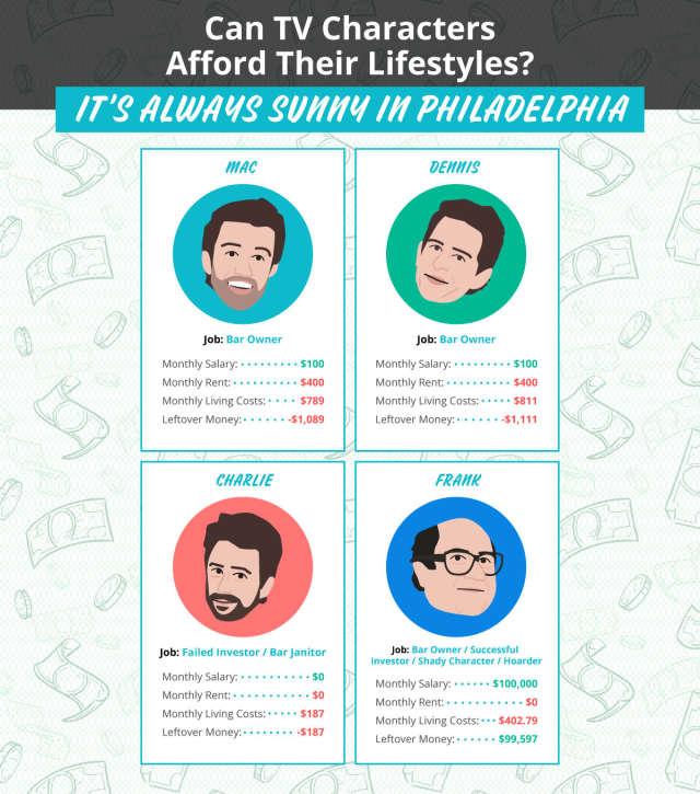
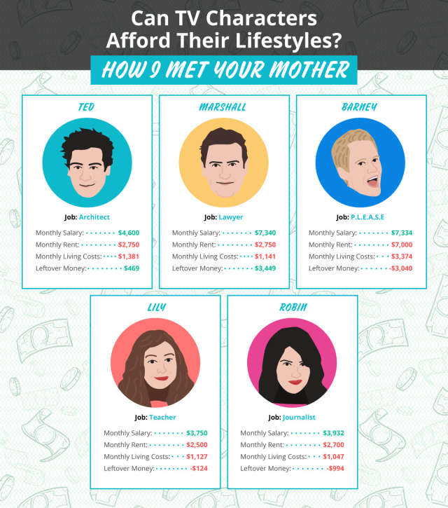
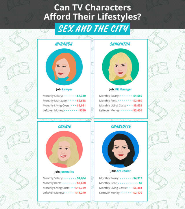
[T]he folks at Joybird decided to dive in a little bit deeper to see which TV characters could actually afford their lifestyles, and they determined that of the 30 characters analyzed, 60 percent could not afford their digs. Let's just say things are a bit more affordable in Hawkins, Indiana than on the Upper East Side.Here are a few of their results:
Friday, October 5, 2018
Thursday, October 4, 2018
Resistance is Futile
In yet another instance of science imitating science fiction, scientists figured out how to create a human hive mind:

A team from the University of Washington (UW) and Carnegie Mellon University has developed a system, known as BrainNet, which allows three people to communicate with one another using only the power of their brain, according to a paper published on the pre-print server arXiv.Pretty cool, but...
In the experiments, two participants (the senders) were fitted with electrodes on the scalp to detect and record their own brainwaves—patterns of electrical activity in the brain—using a method known as electroencephalography (EEG). The third participant (the receiver) was fitted with electrodes which enabled them to receive and read brainwaves from the two senders via a technique called transcranial magnetic stimulation (TMS).
The trio were asked to collaborate using brain-to-brain interactions to solve a task that each of them individually would not be able to complete. The task involved a simplified Tetris-style game in which the players had to decide whether or not to rotate a shape by 180 degrees in order to correctly fill a gap in a line at the bottom of the computer screen.
All of the participants watched the game, although the receiver was in charge of executing the action. The catch is that the receiver was not able to see the bottom half of their screen, so they had to rely on information sent by the two senders using only their minds in order to play.
This system is the first successful demonstration of a “multi-person, non-invasive, direct, brain-to-brain interaction for solving a task,” according to the researchers. There is no reason, they argue, that BrainNet could not be expanded to include as many people as desired, opening up a raft of possibilities for the future.

Thursday, September 27, 2018
All Thumbs
Recently, I was diagnosed with flexor tendinitis in my left thumb. After weeks of pain, I finally saw an orthopedic specialist yesterday, who confirmed the original diagnosis, let me peek at my hand x-rays, and gave me my first (and hopefully last) cortisone injection. It left my thumb puffy, with a rather interesting almond-shaped bruise at the injection point.
If I thought the pain was bad before, it was nothing compared to the pain that showed up about an hour after injection. So severe, I could feel it in my teeth, and I spent the whole day feeling nauseous and jittery from it. Any movement of my thumb was excruciating. I stupidly ordered a dinner that required a knife and fork last night, but I discovered how to hold my fork between my forefinger and middle finger, with my pinky to steady it, much to the amusement of my dinner companion. I'm sure I looked like a kid just learning to use a fork. Who knows? Perhaps that will be a useful skill in the future.
I slept in my thumb brace with my hand resting flat on a pillow, and even still, woke up after every sleep cycle with my hand curled up and on fire.
Today, my thumb is stiff and sore, but I can almost make a fist before it starts to hurt, and I can grasp objects with it for short periods of time. The pain is minimal. It kind of makes yesterday's suffering worth it.
Best case scenario is that this injection cures my tendinitis. Worst case is that it does nothing, but based on how much better I'm feeling, I'm hopeful that isn't what's happening. Somewhere between best and worst case is that I may need another injection in the future. If I keep making a recovery, and feeling better tomorrow, I would probably be willing to do it again. But next time, I'll know not to try going to work after. I was useless and barely able to type.

I'm moving out of my apartment this weekend and I have a draft of a chapter I'm writing due Monday, so sadly, there will probably be no Statistics Sunday post this week. Back to regular posting in October.
Wednesday, September 26, 2018
Thursday, September 20, 2018
On Books, Bad Marketing, and #MeToo
I recently read a book I absolutely loved. Luckiest Girl Alive by Jessica Knoll really got to me and got under my skin in a way few books have. When I went to Goodreads to give the book a 5-star rating, I was shocked at so many negative reviews of 1 and 2 stars. What did I see in this book that others didn't? And what did others see in the book that I didn't?
Nearly all of the negative reviews reference Gone Girl, a fantastic book by one of my new favorite authors, Gillian Flynn. And in fact, Knoll's book had an unfortunate marketing team that sold her book as the "next Gone Girl." Gone Girl this book is not, and that's okay. In fact, it's a bad comparative title, which can break a book. The only thing Ani, the main character in Luckiest Girl Alive has in common with Amy is that they both tried to reinvent themselves to be the type of girl guys like: the cool girl. Oh, and both names begin with A (kind of - Ani's full name is Tifani). That's about it.
While Gone Girl is a twisted tale about the girl Amy pretended to be, manipulating everyone along the way, Luckiest Girl Alive is the case a girl who was drugged and victimized by 4 boys at her school, then revictimized when they turned her classmates against her, calling her all the names we throw so easily at women: slut, skank, an so on. No one believed her, and she was ostracized. She responded by putting as much distance as she could from the events of the past and the person she was, hoping that with the great job, the handsome and rich fiance, designer clothes, and a great body (courtesy of a wedding diet that's little more than an eating disorder), she can move past what happened to her. She becomes bitter and compartmentalized (and also shows many symptoms of PTSD), which may be why some readers didn't like the book and had a hard time dealing with Ani.
I know what's it like to be Ani. Like her, and so many women, I have my own #MeToo story. And I know what it's like to have people I love react like Ani's fiance and mother, who'd rather pretend the events in her past never happened, who change the subject when it's brought up. It's not that we fixate on these things. But those events change us, and when a survivor needs to talk, the people she cares about need to listen, understand, and withhold judgment.
That marketing team failed Jessica Knoll for what should have been a harsh wakeup call in the age of #MeToo, to stop victim blaming. Just like Ani's classmates failed her. And just like nearly everyone close to her failed Amber Wyatt, a survivor of sexual assault who was recently profiled in a Washington Post article (via The Daily Parker).
Given these reactions, it's no wonder many sexual assaults go unreported. Some statistics put that proportion at 80% or higher, with more conservative estimates at 50%. And unfortunately, the proportion of unreported sexual assaults is higher when the victim knows the attacker(s). They're seen as causing trouble, rocking the boat, or trying to save face after regretting a consensual encounter. It's time we start listening to and believing women.

Wednesday, September 19, 2018
The Road Trip That Wasn’t
I was supposed to go to Kansas City today for a visit but sadly it wasn’t meant to be. My car had been sputtering and lurching this morning. When a check engine light came on I pulled off at the nearest exit and headed to the nearest Firestone, which happened to be in Romeoville. I’ve never been though I haven’t missed much, other than a small airport. I got to watch small planes take off and land while I waited for the diagnostic results. It wasn’t spark plugs. Apparently there’s something wrong with the engine. Do not pass go, do not head to Kansas City, go straight to the dealer. Since it’s a Saturn, which they don’t make anymore, that means one of the few GM-authorized dealers that can service Saturns. At least the nice man at Firestone didn’t charge me for the diagnostic reading. They’ll be getting a 5-star review from me.
So I’m staying in Chicago this week/weekend instead of visiting my family. Le sigh.
So I’m staying in Chicago this week/weekend instead of visiting my family. Le sigh.
Tuesday, September 18, 2018
I've Got a Bad Feeling About This
In the 1993 film Jurassic Park, scientist Ian Malcolm expressed serious concern about John Hammond's decision to breed hybrid dinosaurs for his theme park. As Malcolm says in the movie, "No, hold on. This isn't some species that was obliterated by deforestation, or the building of a dam. Dinosaurs had their shot, and nature selected them for extinction."
This movie was, and still is (so far), science fiction. But a team of Russian scientists are working to make something similar into scientific fact:
This movie was, and still is (so far), science fiction. But a team of Russian scientists are working to make something similar into scientific fact:
Long extinct cave lions may be about to rise from their icy graves and prowl once more alongside woolly mammoths and ancient horses in a real life Jurassic Park.Jurassic Park is certainly not the only example of fiction exploring the implications of man "playing god." Many works of literature, like Frankenstein, The Island of Doctor Moreau, and more recent examples like Lullaby (one of my favorites), have examined this very topic. It never ends well.
In less than 10 years it is hoped the fearsome big cats will be released from an underground lab as part of a remarkable plan to populate a remote spot in Russia with Ice Age animals cloned from preserved DNA.
Experiments are already underway to create the lions and also extinct ancient horses found in Yakutia, Siberia, seen as a prelude to restoring the mammoth.
Regional leader Aisen Nikolaev forecast that co-operation between Russian, South Korean and Japanese scientists will see the “miracle” return of woolly mammoths inside ten years.
 |
| By Mauricio Antón - from Caitlin Sedwick (1 April 2008). "What Killed the Woolly Mammoth?". PLoS Biology 6 (4): e99. DOI:10.1371/journal.pbio.0060099., CC BY 2.5, Link |
Sunday, September 16, 2018
Statistics Sunday: What Should I Read Next?
If you're on Goodreads, you can easily download your entire bookshelf, including your to-read books, by going to "My Books" then clicking "Import and Export". On the right side of the screen will be a link for "Export Library". Click that and give it a minute (or several). Soon, a link will appear to download your entire library in a CSV file. You can then bring that into R.
If I'm ever stuck for the next book to read, I can use this file to randomly select a book from my to-read list to check out next. Because I own a lot of books on my to-read list, I'd like to filter that dataset to only include books I own. (Note: You can add books to your "owned" list by clicking on "My Books" then "Owned Books" to select which books you already have in your library. Otherwise, you can keep running the sample function until you get a book you already own or have ready access to. You'd just want to skip the first part of the filter in "reading_list" below.)
setwd("~/Dropbox")
library(tidyverse)
books <- read_csv("goodreads_library_export.csv", col_names = TRUE)
reading_list <- books %>%
  filter(`Owned Copies` == 1, `Exclusive Shelf` == "to-read")
head(reading_list)
## # A tibble: 6 x 31
##   `Book Id` Title    Author  `Author l-f` `Additional Auth… ISBN    ISBN13
##       <int> <chr>    <chr>   <chr>        <chr>             <chr>    <dbl>
## 1  27877138 It       Stephe… King, Steph… <NA>              1501…  9.78e12
## 2     10611 The Eye… Stephe… King, Steph… <NA>              0751…  9.78e12
## 3     11570 Dreamca… Stephe… King, Steph… William Olivier … 2226…  9.78e12
## 4  36452674 The Squ… Kevin … Hearne, Kev… <NA>              <NA>  NA
## 5  38193271 Bickeri… Mildre… Abbott, Mil… <NA>              <NA>  NA
## 6  20873740 Sapiens… Yuval … Harari, Yuv… <NA>              <NA>  NA
## # ... with 24 more variables: `My Rating` <int>, `Average Rating` <dbl>,
## #   Publisher <chr>, Binding <chr>, `Number of Pages` <int>, `Year
## #   Published` <int>, `Original Publication Year` <int>, `Date
## #   Read` <date>, `Date Added` <date>, Bookshelves <chr>, `Bookshelves
## #   with positions` <chr>, `Exclusive Shelf` <chr>, `My Review` <chr>,
## #   Spoiler <chr>, `Private Notes` <chr>, `Read Count` <int>, `Recommended
## #   For` <chr>, `Recommended By` <chr>, `Owned Copies` <int>, `Original
## #   Purchase Date` <chr>, `Original Purchase Location` <chr>,
## #   Condition <chr>, `Condition Description` <chr>, BCID <chr>
Now I have a data frame of books that I own and have not read. This data frame contains 55 books. Drawing a random sample of 1 book is quite easy.
reading_list[sample(1:nrow(reading_list), 1),]
## # A tibble: 1 x 31
##   `Book Id` Title    Author  `Author l-f`  `Additional Auth… ISBN   ISBN13
##       <int> <chr>    <chr>   <chr>         <chr>             <chr>   <dbl>
## 1     14201 Jonatha… Susann… Clarke, Susa… <NA>              0765… 9.78e12
## # ... with 24 more variables: `My Rating` <int>, `Average Rating` <dbl>,
## #   Publisher <chr>, Binding <chr>, `Number of Pages` <int>, `Year
## #   Published` <int>, `Original Publication Year` <int>, `Date
## #   Read` <date>, `Date Added` <date>, Bookshelves <chr>, `Bookshelves
## #   with positions` <chr>, `Exclusive Shelf` <chr>, `My Review` <chr>,
## #   Spoiler <chr>, `Private Notes` <chr>, `Read Count` <int>, `Recommended
## #   For` <chr>, `Recommended By` <chr>, `Owned Copies` <int>, `Original
## #   Purchase Date` <chr>, `Original Purchase Location` <chr>,
## #   Condition <chr>, `Condition Description` <chr>, BCID <chr>
According to this random sample, the next book I should read is Jonathan Strange & Mr Norrell. Now if I'm ever stuck for a book to read, I can use this code to find one. And if I'm in a bookstore, picking up something new - as is often the case, since bookstores are one of my happy places - I can update the code to tell me which book I should buy next.
to_buy <- books %>%
  filter(`Owned Copies` == 0, `Exclusive Shelf` == "to-read")
to_buy[sample(1:nrow(to_buy), 1),]
## # A tibble: 1 x 31
##   `Book Id` Title    Author   `Author l-f` `Additional Aut… ISBN    ISBN13
##       <int> <chr>    <chr>    <chr>        <chr>            <chr>    <dbl>
## 1   2906039 Just Af… Stephen… King, Steph… <NA>             1416…  9.78e12
## # ... with 24 more variables: `My Rating` <int>, `Average Rating` <dbl>,
## #   Publisher <chr>, Binding <chr>, `Number of Pages` <int>, `Year
## #   Published` <int>, `Original Publication Year` <int>, `Date
## #   Read` <date>, `Date Added` <date>, Bookshelves <chr>, `Bookshelves
## #   with positions` <chr>, `Exclusive Shelf` <chr>, `My Review` <chr>,
## #   Spoiler <chr>, `Private Notes` <chr>, `Read Count` <int>, `Recommended
## #   For` <chr>, `Recommended By` <chr>, `Owned Copies` <int>, `Original
## #   Purchase Date` <chr>, `Original Purchase Location` <chr>,
## #   Condition <chr>, `Condition Description` <chr>, BCID <chr>
So next time I'm at a bookstore, which will be tomorrow (since I'll be hanging out in Evanston for a class at my dance studio and plan to hit up the local Barnes & Noble), I should pick up a copy of Just After Sunset.
If you're on Goodreads, feel free to add me!

Saturday, September 15, 2018
Walter Mischel Passes Away
Walter Mischel was an important figure in the history of psychology. His famous "marshmallow study" is still cited and picked apart today. Earlier this week, he passed away from pancreatic cancer. He was 88:

This is a great loss for the field of psychology. But his legacy will live on.
Walter Mischel, whose studies of delayed gratification in young children clarified the importance of self-control in human development, and whose work led to a broad reconsideration of how personality is understood, died on Wednesday at his home in Manhattan. He was 88.
Dr. Mischel was probably best known for the marshmallow test, which challenged children to wait before eating a treat. That test and others like it grew in part out of Dr. Mischel’s deepening frustration with the predominant personality models of the mid-20th century.
“The proposed approach to personality psychology,” he concluded, “recognizes that a person’s behavior changes the situations of his life as well as being changed by them.”
In other words, categorizing people as a collection of traits was too crude to reliably predict behavior, or capture who they are. Dr. Mischel proposed an “If … then” approach to assessing personality, in which a person’s instincts and makeup interact with what’s happening moment to moment, as in: If that waiter ignores me one more time, I’m talking to the manager. Or: If I can make my case in a small group, I’ll do it then, rather than in front of the whole class.
In the late 1980s, decades after the first experiments were done, Dr. Mischel and two co-authors followed up with about 100 parents whose children had participated in the original studies. They found a striking, if preliminary, correlation: The preschoolers who could put off eating the treat tended to have higher SAT scores, and were better adjusted emotionally on some measures, than those who had given in quickly to temptation.
Walter Mischel was born on Feb. 22, 1930, in Vienna, the second of two sons of Salomon Mischel, a businessman, and Lola Lea (Schreck) Mischel, who ran the household. The family fled the Nazis in 1938 and, after stops in London and Los Angeles, settled in the Bensonhurst section of Brooklyn in 1940.
After graduating from New Utrecht High School as valedictorian, Walter completed a bachelor’s degree in psychology at New York University and, in 1956, a Ph.D. from Ohio State University.
He joined the Harvard faculty in 1962, at a time of growing political and intellectual dissent, soon to be inflamed in the psychology department by Timothy Leary and Richard Alpert (a.k.a. Baba Ram Dass), avatars of the era of turning on, tuning in and dropping out.

This is a great loss for the field of psychology. But his legacy will live on.
Thursday, September 13, 2018
Don't Upset a Writer
There's an old joke among writers: don't piss us off. You'll probably end up as an unflattering character or a murder victim in our next project.
There's another joke among writers: if you ever need to bump someone off or dispose of a body, ask a writer. Chances are he or she has thought through a hundred different ways to do it.
The thing about these jokes, though, is that writers usually get our retribution through writing. We don't tend to do the things we write about in real life. If someone legitimately encouraged us to cause real harm to another person or actually help in the commission of a crime, the answer would likely be a resounding "hell no." That's not how we deal with life's slings and arrows. Writing about them is generally enough to satisfy the desire and alleviate the pain.
But not in all cases.
If there were any rules about committing a crime (and I'm sure there are), rule #1 should be: don't write about it on the internet before you do it. And yet, a romance novelist may have done just that. Nancy Crampton Brophy has been charged with murdering her husband; this same author also wrote a blog post called "How to Murder Your Husband":
This year's book will be an adventure/superhero story. And I'm excited to say I'm getting a very clear picture in my head of the story and its key scenes, an important milestone for me if I want to write something I consider good. I didn't have that for last year's project, which is why no one has seen it and I haven't touched it since November 30th. It was by design that I went into it without much prep - that's encouraged for NaNo, to write without bringing out the inner editor. And I'll admit, there are some sections in the book that are beautifully written. I surprised myself, in a good way, with some of it. But all-in-all, it's a mess in need of a LOT of work.

There's another joke among writers: if you ever need to bump someone off or dispose of a body, ask a writer. Chances are he or she has thought through a hundred different ways to do it.
The thing about these jokes, though, is that writers usually get our retribution through writing. We don't tend to do the things we write about in real life. If someone legitimately encouraged us to cause real harm to another person or actually help in the commission of a crime, the answer would likely be a resounding "hell no." That's not how we deal with life's slings and arrows. Writing about them is generally enough to satisfy the desire and alleviate the pain.
But not in all cases.
If there were any rules about committing a crime (and I'm sure there are), rule #1 should be: don't write about it on the internet before you do it. And yet, a romance novelist may have done just that. Nancy Crampton Brophy has been charged with murdering her husband; this same author also wrote a blog post called "How to Murder Your Husband":
Crampton Brophy, 68, was arrested Sept. 5 on charges of murdering her husband with a gun and unlawful use of a weapon in the death of her husband, Daniel Brophy, according to the Portland Police Bureau.It's kind of surprising to me that Brophy's books are romances and yet apparently involve a lot of murder and death. I don't read romance, so maybe murder and death is a common theme and I just don't know it. Of course, as I was thinking about last year's NaNoWriMo book, I surprised myself when I realized that the genre may, in fact, be romance. One without any murder, though.
The killing puzzled police and those close to Daniel Brophy from the start. Brophy, a 63-year-old chef, was fatally shot at his workplace at the Oregon Culinary Institute on the morning of June 2. Students were just beginning to file into the building for class when they found him bleeding in the kitchen, KATU2 news reported. Police had no description of the suspect.
In Crampton Brophy’s “How to Murder Your Husband” essay, she had expressed that although she frequently thought about murder, she didn’t see herself following through with something so brutal. She wrote she would not want to “worry about blood and brains splattered on my walls,” or “remembering lies.”
“I find it easier to wish people dead than to actually kill them,” she wrote. “. . . But the thing I know about murder is that every one of us have it in him/her when pushed far enough.”
This year's book will be an adventure/superhero story. And I'm excited to say I'm getting a very clear picture in my head of the story and its key scenes, an important milestone for me if I want to write something I consider good. I didn't have that for last year's project, which is why no one has seen it and I haven't touched it since November 30th. It was by design that I went into it without much prep - that's encouraged for NaNo, to write without bringing out the inner editor. And I'll admit, there are some sections in the book that are beautifully written. I surprised myself, in a good way, with some of it. But all-in-all, it's a mess in need of a LOT of work.

Tuesday, September 11, 2018
Inside the Nike Call Center
One more post before I leave work for the day - Rolling Stone interviewed an employee of the Nike call center, who requested he remain anonymous. His responses are interesting, though sadly not surprising:
So, what has this week been like for you?
Bittersweet. A lot of us have more respect for our company than we have in the past. We feel a big swell of pride that we stood up for something meaningful. But we’ve been getting harassed like crazy.
Normally it’s like whatever, I’m getting paid for it. But this week hit home. With any job you’re going to have to deal with some abuse. Sometimes you can just go with it and apologize, but with this there was no reasoning with it. It felt like it was the proverbial klan’s mask: looking at someone and not knowing their identity, wanting to take off the mask, but you’re getting your ass whooped so you can’t.
What about donating?
Only one group of people called to say they were donating.
A group of republican moms told me they meet up to talk about local news and politics and because of this they have stopped all their support of Nike. They said, “We gathered up all our kids’ Nike stuff and we’re going to go donate it. All our kids play sports but will find another brand.”
I said “Wow, that’s really nice. That’s good. I’m happy for you.”
They basically said, “F*** you, it’s not funny. We’re never going to give another cent, we’re going to talk to our brokers and withdraw our stock.”
No Take Bachs
About a week ago, Boing Boing published a story with a shocking claim: you can't post performance videos of Bach's music because Sony owns the compositions.
Wait, what?
Automation is being added to this and many related cases to take out the bias of human judgment. This leads to a variety of problems with technology running rampant and affecting lives, as has been highlighted in recent books like Weapons of Math Destruction and Technically Wrong.
A human being watching Rhodes's video would be able to tell right away that no copyright infringement took place. Rhodes was playing the same composition played in a performance owned by Sony - it's the same source material, which is clearly in the public domain, rather than the same recording, which is not public domain.
This situation is also being twisted into a way to make money:

Wait, what?
James Rhodes, a pianist, performed a Bach composition for his Facebook account, but it didn't go up -- Facebook's copyright filtering system pulled it down and accused him of copyright infringement because Sony Music Global had claimed that they owned 47 seconds' worth of his personal performance of a song whose composer has been dead for 300 years.You don't need to be good at math to know that this claim must be false. Sony can't possibly own compositions that are clearly in the public domain. What this highlights though is that something, while untrue in theory, can be true in practice. Free Beacon explains:
As it happens, the company genuinely does hold the copyright for several major Bach recordings, a collection crowned by Glenn Gould's performances. The YouTube claim was not that Sony owned Bach's music in itself. Rather, YouTube conveyed Sony's claim that Rhodes had recycled portions of a particular performance of Bach from a Sony recording.Does Sony own copyright on Bach in theory? No, absolutely not. But this system, which scans for similarity in the audio, is making this claim true in practice: performers of Bach's music will be flagged automatically by the system as using copyrighted content, and attacked with take-down notices and/or having their videos deleted altogether. There's only so much one can do with interpretation and tempo to change the sound, and while skill of the performer will also impact the audio, to a computer, the same notes and same tempo will sound the same.
The fact that James Rhodes was actually playing should have been enough to halt any sane person from filing the complaint. But that's the real point of the story. No sane person was involved, because no actual person was involved. It all happened mechanically, from the application of the algorithms in Youtube's Content ID system. A crawling bot obtained a complex digital signature for the sound in Rhodes's YouTube posting. The system compared that signature to its database of registered recordings and found a partial match of 47 seconds. The system then automatically deleted the video and sent a "dispute claim" to Rhodes's YouTube channel. It was a process entirely lacking in human eyes or human ears. Human sanity, for that matter.
Automation is being added to this and many related cases to take out the bias of human judgment. This leads to a variety of problems with technology running rampant and affecting lives, as has been highlighted in recent books like Weapons of Math Destruction and Technically Wrong.
A human being watching Rhodes's video would be able to tell right away that no copyright infringement took place. Rhodes was playing the same composition played in a performance owned by Sony - it's the same source material, which is clearly in the public domain, rather than the same recording, which is not public domain.
This situation is also being twisted into a way to make money:
[T]he German music professor Ulrich Kaiser wanted to develop a YouTube channel with free performances for teaching classical music. The first posting "explained my project, while examples of the music played in the background. Less than three minutes after uploading, I received a notification that there was a Content ID claim against my video." So he opened a different YouTube account called "Labeltest" to explore why he was receiving claims against public-domain music. Notices from YouTube quickly arrived for works by Bartok, Schubert, Puccini, Wagner, and Beethoven. Typically, they read, "Copyrighted content was found in your video. The claimant allows its content to be used in your YouTube video. However, advertisements may be displayed."
And that "advertisements may be displayed" is the key. Professor Kaiser wanted an ad-free channel, but his attempts to take advantage of copyright-free music quickly found someone trying to impose advertising on him—and thereby to claim some of the small sums that advertising on a minor YouTube channel would generate.
Last January, an Australian music teacher named Sebastian Tomczak had a similar experience. He posted on YouTube a 10-hour recording of white noise as an experiment. "I was interested in listening to continuous sounds of various types, and how our perception of these kinds of sounds and our attention changes over longer periods," he wrote of his project. Most listeners would probably wonder how white noise, chaotic and random by its nature, could qualify as a copyrightable composition (and wonder as well how anyone could get through 10 hours of it). But within days, the upload had five different copyright claims filed against it. All five would allow continued use of the material, the notices explained, if Tomczak allowed the upload to be "monetized," meaning accompanied by advertisements from which the claimants would get a share.

Monday, September 10, 2018
Dolphin Superpods
A thousand dolphins gathered in Monterey Bay, California, hunting for bait fish. While this gathering - like a dolphin food festival - usually happens farther from shore, this gathering happened closer to the coastline, allowing a rare glimpse of the dolphin superpod:
Sunday, September 9, 2018
150 Years in Chicago
This morning, I joined some of my musician friends to sing for a mass celebrating the 150th anniversary of St. Thomas the Apostle in Hyde Park, Chicago. In true music-lover fashion, the mass was also part concert, featuring some gorgeous choral works, including:

- Kyrie eleison from Vierne's Messe Solennelle: my choir is performing this work in our upcoming season, and I give 4 to 1 odds that this movement, the Kyrie, ends up in our Fall Preview concert (which I unfortunately won't be singing, due to a work commitment)
- Locus iste by Bruckner
- Thou knowest, Lord by Purcell
- Ave Verum Corpus by Mozart
- Amen from Handel's Messiah (which my choir performs every December)
The choir was small but mighty - 3 sopranos, 4 altos, 4 tenors, and 5 basses - and in addition to voices, we had violin, trumpet, cello, and organ. The music was gorgeous. Afterward, I ate way too much food at the church picnic.
I'm tempted to take an afternoon nap. Instead, I'll be packing up my apartment.
Statistics Sunday: What is Standard Setting?
In a past post, I talked about content validation studies, a big part of my job. Today, I'm going to give a quick overview of standard setting, another big part of my job, and an important step in many testing applications.
In any kind of ability testing application, items will be written with identified correct and incorrect answers. This means you can generate overall scores for your examinees, whether the raw score is simply the number of correct answers or generated with some kind of item response theory/Rasch model. But what isn't necessarily obvious is how to use those scores to categorize candidates and, in credentialing and similar applications, who should pass and who should fail.
This is the purpose of standard setting: to identify cut scores for different categories, such as pass/fail, basic/proficient/advanced, and so on.
There are many different methods for conducting standard setting. Overall, approaches can be thought of as item-based or holistic/test-based.
For item-based methods, standard setting committee members go through each item and categorize it in some way (the precise way depends on which method is being used). For instance, they may categorize it as basic, proficient, or advanced, or they may generate the likelihood that a minimally qualified candidate (i.e., the person who should pass) would get it right.
For holistic/test-based methods, committee members make decisions about cut scores within the context of the whole test. Holistic/test-based methods still require review of the entire exam, but don't require individual judgments about each item. For instance, committee members may have a booklet containing all items in order of difficulty (based on pretest data), and place a bookmark at the item that reflects the transition from proficient to advanced or from fail to pass.
The importance of standard setting comes down to defensibility. In licensure, for instance, failing a test may mean being unable to work in one's field at all. For this reason, definitions of who should pass and who should fail (in terms of knowledge, skills, and abilities) should be very strong and clearly tied to exam scores. And licensure and credentialing organizations are frequently required to prove, in a court of law, that their standards are fair, rigorously derived, and meaningful.
For my friends and readers in academic settings, this step may seem unnecessary. After all, you can easily categorize students into A, B, C, D, and F with the percentage of items correct. But this is simply a standard (that is, the cut score for pass/fail is 60%), set at some point in the past, and applied through academia.
I'm currently working on a chapter on standard setting with my boss and a coworker. And for anyone wanting to learn more about standard setting, two great books are Cizek and Bunch's Standard Setting and Zieky, Perie, and Livingston's Cut Scores.
Wednesday, September 5, 2018
Lots of Writing, Just Not On the Blog
Hi all! Again, it's been a while since I've blogged something. I'm currently keeping busy with multiple writing projects, and I'm hoping to spin one of them into a blog post soon:

- I'm still analyzing a huge survey dataset for my job, and writing up new analyses requested by our boards and advisory councils, as well as creating a version for laypeople (i.e., general public as opposed to people with a stats/research background)
- My team submitted to write a chapter for the 3rd edition of The Institute for Credentialing Excellence Handbook, an edited volume about important topics in credentialing/high-stakes testing; I'm leading our chapter on standard setting, which cover methods for standard setting (selecting exam pass points) and the logistics of conducting a standard-setting study
- I've already begun research for my NaNoWriMo novel, which will be a superhero story, so elements of sci-fi and fantasy and lots of fun world-building
- Lastly, I'm developing two new surveys, one for a content validation study and the other a regular survey we send out to assess the dental assisting workforce

Thursday, August 30, 2018
Today's Reading List
I'm wrapping up a few department requests as we head into the end of our fiscal year, so these tabs will have to wait until later:

- The (I think) repulsive Red Delicious apple has finally dropped from its spot as Dominant Apple in the US, to be replaced by the Gala apple. But don't worry, Red Delicious lovers, it's still number 2. My favorite, Granny Smith, is number 3.
- CityLab tracks the rise of Andrew Gillum, first African-American Democratic nominee for Florida governor.
- Also on CityLab, staffers share their best and worst roommate stories
- The Daily Parker drops a Hitchhiker's Guide reference regarding a story of a commissioned mural that was mistaken for graffiti and destroyed
- And finally, the 5 books every data scientist should read (that are not about data science)
Back to work.

Monday, August 27, 2018
Statistics Sunday: Visualizing Regression
To demonstrate this technique, I'm using my 2017 reading dataset. A reader requested I make this dataset available, which I have done - you can download it here. This post describes the data in more detail, but the short description is that this dataset contains the 53 books I read last year, with information on book genre, page length, how long it took me to read it, and two ratings: my own rating and the average rating on Goodreads. Look for another dataset soon, containing my 2018 reading data; I made a goal of 60 books and I've already read 50, meaning lots more data than last year. I'm thinking of going for broke and bumping my reading goal up to 100, because apparently 60 books is not enough of a challenge for me now that I spend so much downtime reading.
First, I'll load my dataset, then conduct the basic linear model I demonstrated in the post linked above.
setwd("~/R")
library(tidyverse)
## Warning: Duplicated column names deduplicated: 'Author' => 'Author_1' [13]
colnames(books)[13] <- "Author_Gender"
myrating<-lm(My_Rating ~ Pages + Read_Time + Author_Gender + Fiction + Fantasy + Math_Stats + YA_Fic, data=books)
summary(myrating)
##
## Call:
## lm(formula = My_Rating ~ Pages + Read_Time + Author_Gender +
##     Fiction + Fantasy + Math_Stats + YA_Fic, data = books)
##
## Residuals:
##      Min       1Q   Median       3Q      Max
## -0.73120 -0.34382 -0.00461  0.24665  1.49932
##
## Coefficients:
##                 Estimate Std. Error t value Pr(>|t|)
## (Intercept)    3.5861211  0.2683464  13.364   <2e-16 ***
## Pages          0.0019578  0.0007435   2.633   0.0116 *
## Read_Time     -0.0244168  0.0204186  -1.196   0.2380
## Author_Gender -0.1285178  0.1666207  -0.771   0.4445
## Fiction        0.1052319  0.2202581   0.478   0.6351
## Fantasy        0.5234710  0.2097386   2.496   0.0163 *
## Math_Stats    -0.2558926  0.2122238  -1.206   0.2342
## YA_Fic        -0.7330553  0.2684623  -2.731   0.0090 **
## ---
## Signif. codes:  0 '***' 0.001 '**' 0.01 '*' 0.05 '.' 0.1 ' ' 1
##
## Residual standard error: 0.4952 on 45 degrees of freedom
## Multiple R-squared:  0.4624, Adjusted R-squared:  0.3788
## F-statistic:  5.53 on 7 and 45 DF,  p-value: 0.0001233
These analyses show that I give higher ratings for books that are longer and Fantasy genre, and lower ratings to books that are Young Adult Fiction. Now let's see what happens if I run this same linear model through rpart. Note that this is a slightly different technique, looking for cuts that differentiate outcomes, so it will find slightly different results.
library(rpart)
tree1 <- rpart(My_Rating ~ Pages + Read_Time + Author_Gender + Fiction + Fantasy + Math_Stats + YA_Fic, method = "anova", data=books)
printcp(tree1)
##
## Regression tree:
## rpart(formula = My_Rating ~ Pages + Read_Time + Author_Gender +
##     Fiction + Fantasy + Math_Stats + YA_Fic, data = books, method = "anova")
##
## Variables actually used in tree construction:
## [1] Fantasy    Math_Stats Pages
##
## Root node error: 20.528/53 = 0.38733
##
## n= 53
##
##         CP nsplit rel error  xerror    xstd
## 1 0.305836      0   1.00000 1.03609 0.17531
## 2 0.092743      1   0.69416 0.76907 0.12258
## 3 0.022539      2   0.60142 0.71698 0.11053
## 4 0.010000      3   0.57888 0.74908 0.11644
These results differ somewhat. Pages is still a significant variable, as is Fantasy. But now Math_Stats (indicating books that are about mathematics or statistics, one of my top genres from last year) also is. These are the variables used by the analysis to construct my regression tree. If we look at the full summary -
summary(tree1)
## Call:
## rpart(formula = My_Rating ~ Pages + Read_Time + Author_Gender +
##     Fiction + Fantasy + Math_Stats + YA_Fic, data = books, method = "anova")
##   n= 53
##
##           CP nsplit rel error    xerror      xstd
## 1 0.30583640      0 1.0000000 1.0360856 0.1753070
## 2 0.09274251      1 0.6941636 0.7690729 0.1225752
## 3 0.02253938      2 0.6014211 0.7169813 0.1105294
## 4 0.01000000      3 0.5788817 0.7490758 0.1164386
##
## Variable importance
##      Pages    Fantasy    Fiction     YA_Fic Math_Stats  Read_Time
##         62         18          8          6          4          3
##
## Node number 1: 53 observations,    complexity param=0.3058364
##   mean=4.09434, MSE=0.3873265
##   left son=2 (9 obs) right son=3 (44 obs)
##   Primary splits:
##       Pages         < 185 to the left,  improve=0.30583640, (0 missing)
##       Fiction       < 0.5 to the left,  improve=0.24974560, (0 missing)
##       Fantasy       < 0.5 to the left,  improve=0.20761810, (0 missing)
##       Math_Stats    < 0.5 to the right, improve=0.20371790, (0 missing)
##       Author_Gender < 0.5 to the right, improve=0.02705187, (0 missing)
##
## Node number 2: 9 observations
##   mean=3.333333, MSE=0.2222222
##
## Node number 3: 44 observations,    complexity param=0.09274251
##   mean=4.25, MSE=0.2784091
##   left son=6 (26 obs) right son=7 (18 obs)
##   Primary splits:
##       Fantasy    < 0.5 to the left,  improve=0.15541600, (0 missing)
##       Fiction    < 0.5 to the left,  improve=0.12827990, (0 missing)
##       Math_Stats < 0.5 to the right, improve=0.10487750, (0 missing)
##       Pages      < 391 to the left,  improve=0.05344995, (0 missing)
##       Read_Time  < 7.5 to the right, improve=0.04512078, (0 missing)
##   Surrogate splits:
##       Fiction   < 0.5 to the left,  agree=0.773, adj=0.444, (0 split)
##       YA_Fic    < 0.5 to the left,  agree=0.727, adj=0.333, (0 split)
##       Pages     < 370 to the left,  agree=0.682, adj=0.222, (0 split)
##       Read_Time < 3.5 to the right, agree=0.659, adj=0.167, (0 split)
##
## Node number 6: 26 observations,    complexity param=0.02253938
##   mean=4.076923, MSE=0.2248521
##   left son=12 (7 obs) right son=13 (19 obs)
##   Primary splits:
##       Math_Stats    < 0.5 to the right, improve=0.079145230, (0 missing)
##       Pages         < 364 to the left,  improve=0.042105260, (0 missing)
##       Fiction       < 0.5 to the left,  improve=0.042105260, (0 missing)
##       Read_Time     < 5.5 to the left,  improve=0.016447370, (0 missing)
##       Author_Gender < 0.5 to the right, improve=0.001480263, (0 missing)
##
## Node number 7: 18 observations
##   mean=4.5, MSE=0.25
##
## Node number 12: 7 observations
##   mean=3.857143, MSE=0.4081633
##
## Node number 13: 19 observations
##   mean=4.157895, MSE=0.132964
we see that Fiction, YA_Fic, and Read_Time were also significant variables. The problem is that there is multicollinearity between Fiction, Fantasy, Math_Stats, and YA_Fic. All Fantasy and YA_Fic books are Fiction, while all Math_Stats books are not Fiction. And all YA_Fic books I read were Fantasy. This is probably why the tree didn't use Fiction or YA_Fic. I'm not completely clear on why Read_Time didn't end up in the regression tree, but it may be because my read time was pretty constant among the different splits and didn't add any new information to the tree. If I were presenting these results somewhere other than my blog, I'd probably want to do some follow-up analyses to confirm this fact.
Now the fun part: let's plot our regression tree:
plot(tree1, uniform = TRUE, main = "Regression Tree for My Goodreads Ratings")
text(tree1, use.n = TRUE, all = TRUE, cex = 0.8)

While this plot is great for a quick visualization, I can make a nicer looking plot (which doesn't cut off the bottom text) as a PostScript file.
post(tree1, file = "mytree.ps",
        title = "Regression Tree for Rating")
I converted that to a PDF, which you can view here.
Hope you enjoyed this post! Have any readers used this technique before? Any thoughts or applications you'd like to share? (Self-promotion highly encouraged!)
Subscribe to:
Posts (Atom)