.png)
Tuesday, May 8, 2018


Monday, May 7, 2018
New Database, Who Dis?
Next week, my company is launching a new database to maintain our many records: anyone who has taken one of our exams, certificants (people who have completed sets of exams that entitle them to a certificate), schools, companies, and so on. Our old system, which I found out today is 20 years old, goes down Wednesday evening, and then we'll begin transferring over 4 million records into the new system. (We've done some test runs of transferring data and extensive mapping for many months now. And I've been scoring and QCing exams in a Dev environment for almost that long.)
It's been a long, busy process to get to this point, working with multiple vendors, and I've been spending the last several months preparing us to score our exams in the new system. This project has been good practice for, among other things, understanding how we convert Rasch scores to our standard scaling, how we create item strings for scoring computer adaptive exams, and keeping my SQL skills fresh. And since I'm currently a one-person department, as a coworker is out on maternity leave and another left to take another job, I'm completing job tasks for 2.5 to 3 people every day, on top of database stuff.
Blogging will likely be on hold this week and I may not have a Statistics Sunday post, since I'll be working all-day Saturday and most/all of Sunday. But I'll see if I can squeeze some time in for something.

It's been a long, busy process to get to this point, working with multiple vendors, and I've been spending the last several months preparing us to score our exams in the new system. This project has been good practice for, among other things, understanding how we convert Rasch scores to our standard scaling, how we create item strings for scoring computer adaptive exams, and keeping my SQL skills fresh. And since I'm currently a one-person department, as a coworker is out on maternity leave and another left to take another job, I'm completing job tasks for 2.5 to 3 people every day, on top of database stuff.
Blogging will likely be on hold this week and I may not have a Statistics Sunday post, since I'll be working all-day Saturday and most/all of Sunday. But I'll see if I can squeeze some time in for something.

Sunday, May 6, 2018
Statistics Sunday: Tokenizing Text
In text analysis, a token is any kind of meaningful text unit that can be analyzed. Frequently, a token is a word and the process of tokenizing splits up the text into individual words and counts up how many times each word appears in the text. But a token could also be a phrase (such as each two-word combination present in a text, which is called a bi-gram), a sentence, a paragraph, even a whole chapter. Obviously, the size of the token you choose impacts what kind of analysis you can do. Generally, people choose smaller tokens, like words.
Let's use R to download the text of a classic book (which I did previously in this post, but today, I'll do in an easier way) and tokenize it by word.
Any text available in the Project Gutenberg repository can be downloaded, with header and footer information stripped out, with the guternbergr package.
install.packages("gutenbergr")
library(gutenbergr)
The package comes with a dataset, called gutenberg_metadata, that contains a list, by ID, of all text available. Let's use The War of the Worlds by H.G. Wells as our target book. We can find our target book like this:
library(tidyverse)
gutenberg_metadata %>%
  filter(title == "The War of the Worlds")
## # A tibble: 3 x 8
##   gutenberg_id title   author   gutenberg_autho… language gutenberg_books…
##          <int> <chr>   <chr>               <int> <chr>    <chr>
## 1           36 The Wa… Wells, …               30 en       Movie Books/Sci…
## 2         8976 The Wa… Wells, …               30 en       Movie Books/Sci…
## 3        26291 The Wa… Wells, …               30 en       <NA>
## # ... with 2 more variables: rights <chr>, has_text <lgl>
The ID for The War of the Worlds is 36. Now I can use that information to download the text of the book into a data frame, using the gutenbergr function, gutenberg_download.
warofworlds<-gutenberg_download(36)
Now I have a dataset with two variables: one containing the Project Gutenberg ID for the text (which is helpful if you create a dataset with multiple texts, perhaps all by the same author or within the same genre) and one containing a line of text. To tokenize our dataset, we need the R package, tidytext.
install.packages("tidytext")
library(tidytext)
We can tokenize with the function, unnest_tokens: first we tell it to do so by word then we tell it which column to look in to find the tokens.
tidywow<-warofworlds %>%
  unnest_tokens(word, text)
Now we have a dataset with each word from the book, one after the other. There are duplicates in here, because I haven't told R to count up the words. Before I do that, I probably want to tell R to ignore extremely common words, like "the," "and," "to," and so on. In text analysis, these are called stop words, and tidytext comes with a dataset called stop_words that can be used to drop stop words from your text data.
tidywow<-tidywow %>%
  anti_join(stop_words)
Last, we have R count up the words.
wowtokens<-tidywow %>%
  count(word, sort=TRUE)
head(wowtokens)
## # A tibble: 6 x 2
##   word         n
##   <chr>    <int>
## 1 martians   163
## 2 people     159
## 3 black      122
## 4 time       121
## 5 road       104
## 6 night      102
After removing stop words, of which there may be hundreds or thousands in any text, the most common words are: Martians, people, black, time, and road.

Thursday, May 3, 2018
The Pillars of Creation
About 7,000 light years away are the Pillars of Creation, a collection of clouds and dust in the Eagle Nebula. Inside the pillars, gravity works to pull the gas onto new and existing stars, while heat from internal and external stars expel and evaporate the gas. The picture (actually a composite of many pictures) of the pillars taken in 1995 is perhaps one of the most famous pictures of objects in space:
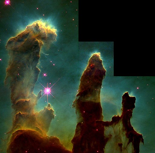
In 2007, NASA released the results of a study saying the Pillars of Creation were toppled about 6,000 years ago, when a star went supernova about 8,000 years ago, destroying the pillars over the next 2,000 years. Because the pillars are 7,000 light years away, we won't be able to see that they've been destroyed for another 1,000 years.
However, an article by Ethan Siegel suggests the pillars have not been destroyed after all:

Time to witness another great instance of birth/rebirth - the editing of a Wikipedia article. When I checked just now, the nebula article still states the pillars have been destroyed. Let's see how long it takes for that to change:


In 2007, NASA released the results of a study saying the Pillars of Creation were toppled about 6,000 years ago, when a star went supernova about 8,000 years ago, destroying the pillars over the next 2,000 years. Because the pillars are 7,000 light years away, we won't be able to see that they've been destroyed for another 1,000 years.
However, an article by Ethan Siegel suggests the pillars have not been destroyed after all:
At 7,000 light years away, the Eagle Nebula is one of the night sky’s most accessible and spectacular nebulae. It was discovered back in 1745, and shortly thereafter was recognized to be an active star-forming region, as the surefire signature of ionized hydrogen was seen in abundance. A large cluster of newborn stars can be found inside, consisting of over 8,000 stars, which is the primary cause of the nebula’s shape.Here's how the pillars looked in the 2015 photo:
[I]n 2015, to celebrate Hubble’s 25th anniversary in space, NASA revisited these pillars, and the 20 year baseline between the original 1995 image and the new 2015 one provided insights that strongly refuted the already-destroyed pillars theory.
The 20-year follow-up showcased not only features that couldn’t be seen before, such as additional details, greater wavelength coverage, and a larger field of view. But the greatest and most important advance is the fact that the 20-year baseline allowed us to view changes over time. In the tip of the largest pillar, for example, we were able to not only identify an ejected jet, but to track the extent of its changes. With the incredible resolution of Hubble, we could determine that the size of it, over that additional time, expanded by an extra 100 billion kilometers: 1000 times the Earth-Sun distance, meaning that the stream is moving at 200 km/s.
Moreover, the best evidence for changes comes at the base of the pillars, indicating an evaporation time on the order of between 100,000 and 1,000,000 years. The idea that the pillars have already been destroyed has been demonstrated not to be true. It’s one of the great hopes of science that any controversial claims will be laid to rest by more and better data, and this is one situation where that has paid off in spades. Not only has there not been a supernova that’s in the process of destroying the pillars, but the pillars themselves should be robust for a long time to come.

Time to witness another great instance of birth/rebirth - the editing of a Wikipedia article. When I checked just now, the nebula article still states the pillars have been destroyed. Let's see how long it takes for that to change:

Wednesday, May 2, 2018
Statistical Sins: Is Your Classification Model Any Good?
Specifically, I talked a couple of times about binomial regression (here and here), which is used to predict (read: recreate with a set of variables significantly related to) a binary outcome. The data example I used involved my dissertation data and the binary outcome was verdict: guilty or not guilty. A regression model returns the linear correction applied to the predictor variables to reproduce the outcome, and will highlight whether a predictor was significantly related to the outcome or not. But a big question you may be asking of your binomial model is: how well does it predict the outcome? Specifically, how can you examine whether your regression model is correctly classifying cases?
We'll start by loading/setting up the data and rerunning the binomial regression with interactions.
dissertation<-read.delim("dissertation_data.txt",header=TRUE)
dissertation<-dissertation[,1:44]
predictors<-c("obguilt","reasdoubt","bettertolet","libertyvorder",
              "jurevidence","guilt")
dissertation<-subset(dissertation, !is.na(libertyvorder))

dissertation[45:50]<-lapply(dissertation[predictors], function(x) {
  y<-scale(x, center=TRUE, scale=TRUE)
  }
)

pred_int<-'verdict ~ obguilt.1 + reasdoubt.1 + bettertolet.1 + libertyvorder.1 +
                  jurevidence.1 + guilt.1 + obguilt.1*guilt.1 + reasdoubt.1*guilt.1 +
                  bettertolet.1*guilt.1 + libertyvorder.1*guilt.1 + jurevidence.1*guilt.1'
model<-glm(pred_int, family="binomial", data=dissertation)
summary(model)
##
## Call:
## glm(formula = pred_int, family = "binomial", data = dissertation)
##
## Deviance Residuals:
##     Min       1Q   Median       3Q      Max
## -2.6101  -0.5432  -0.1289   0.6422   2.2805
##
## Coefficients:
##                         Estimate Std. Error z value Pr(>|z|)
## (Intercept)             -0.47994    0.16264  -2.951  0.00317 **
## obguilt.1                0.25161    0.16158   1.557  0.11942
## reasdoubt.1             -0.09230    0.20037  -0.461  0.64507
## bettertolet.1           -0.22484    0.20340  -1.105  0.26899
## libertyvorder.1          0.05825    0.21517   0.271  0.78660
## jurevidence.1            0.07252    0.19376   0.374  0.70819
## guilt.1                  2.31003    0.26867   8.598  < 2e-16 ***
## obguilt.1:guilt.1        0.14058    0.23411   0.600  0.54818
## reasdoubt.1:guilt.1     -0.61724    0.29693  -2.079  0.03764 *
## bettertolet.1:guilt.1    0.02579    0.30123   0.086  0.93178
## libertyvorder.1:guilt.1 -0.27492    0.29355  -0.937  0.34899
## jurevidence.1:guilt.1    0.27601    0.36181   0.763  0.44555
## ---
## Signif. codes:  0 '***' 0.001 '**' 0.01 '*' 0.05 '.' 0.1 ' ' 1
##
## (Dispersion parameter for binomial family taken to be 1)
##
##     Null deviance: 490.08  on 354  degrees of freedom
## Residual deviance: 300.66  on 343  degrees of freedom
## AIC: 324.66
##
## Number of Fisher Scoring iterations: 6
The predict function, which I introduced here, can also be used for the binomial model. Let's have R generate predicted scores for everyone in the dissertation sample:
dissertation$predver<-predict(model)
dissertation$predver
##   [1]  0.3907097456 -4.1351129605  2.1820478279 -2.8768390246  2.5804618523
##   [6]  0.4244692909  2.3065468369 -2.7853434926  0.3504760502 -0.2747339639
##  [11] -1.8506160725 -0.6956240161 -4.7860574839 -0.3875950731 -2.4955679446
##  [16] -0.3941516951 -4.5831011509  1.6185480937  0.4971923298  4.1581842900
##  [21] -0.6320531052 -4.8447046319 -2.3974890696  1.8566258698  0.0360685822
##  [26]  2.2151040131  2.3477149003 -2.4493726369 -0.2253481404 -4.8899805287
##  [31]  1.7789459288 -0.0978703861 -3.5541042186 -3.6009218603  0.1568318789
##  [36]  3.7866003489 -0.6371816898 -0.7047761441 -0.7529742376 -0.0302759317
##  [41] -0.1108055330  1.9751810033  0.2373614802  0.0424471071 -0.4018757856
##  [46]  0.0530272726 -1.0763759980  0.0099577637  0.3128581222  1.4806679691
##  [51] -1.7468626219  0.2998282372 -3.6359162016 -2.2200774510  0.3192366472
##  [56]  3.0103216033 -2.0625775984 -6.0179845235  2.0300503627  2.3676828409
##  [61] -2.8971753746 -3.2131490026  2.1349358889  3.0215336139  1.2436192890
##  [66]  0.2885535375  0.2141821004  1.9480686936  0.0438751446 -1.9368013875
##  [71]  0.2931258287  0.5319938265  0.0177643261  3.3724920900  0.0332949791
##  [76]  2.5935500970  0.7571810150  0.7131757400  2.5411073339  2.8499853550
##  [81]  2.8063291084 -0.4500738791  1.4700679077 -0.8659309719  0.0870492258
##  [86]  0.5728074322  0.1476797509  2.4697257261  2.5935500970 -2.2200774510
##  [91] -0.0941827753  1.3708676633  1.4345235392 -0.2407209578  2.4662700339
##  [96] -1.9687731888 -6.7412580522 -0.0006224018 -4.4132951092 -2.8543032695
## [101]  1.2295635352  2.8194173530  0.1215689324 -3.8258079371  1.8959803882
## [106] -4.5578801595  2.3754402614  0.0826808026  1.5112359711 -3.5402060466
## [111]  0.2556657363  0.7054183194  1.4675797244 -2.3974890696  2.6955929822
## [116] -0.3123518919 -4.8431862346 -2.0132721372  0.4673405434 -2.3053405270
## [121]  1.9498822386 -0.5164183930 -1.8277820872 -0.0134750769 -2.3013547136
## [126] -0.2498730859 -4.4281010683 -0.0134750769 -0.2604532514  0.1476797509
## [131] -2.3392939519 -2.0625775984 -3.5541042186  1.5087477879 -4.6453051124
## [136]  2.0616474606 -3.2691362859 -7.3752231145 -1.6666447439  1.0532964013
## [141] -2.0625775984 -0.3355312717  2.2481601983 -2.2200774510 -4.3276959075
## [146]  0.8685972087 -0.7727065311  1.7511589809 -0.4774548995  0.0008056357
## [151]  1.7022334970 -0.4202625135 -0.2902646169  2.4409712692  0.0008056357
## [156]  0.0008056357 -3.6009218603 -0.8567788439 -0.4528474822  0.3517462520
## [161]  0.1307210605 -3.7843118182 -2.8419024763 -3.5191098774 -0.1460684795
## [166]  1.8809888141  2.8194173530 -2.4656469123  1.0589888029  0.1659840070
## [171]  1.4345235392  2.3676828409  1.5749534339 -0.1681557545  2.6406620359
## [176]  0.1476797509 -2.2135177411  1.9168260534 -3.4993205379  0.4557086940
## [181] -3.8136089417 -0.1121510987 -3.9772095600  1.3849234171  0.3504760502
## [186]  2.3807710856 -3.0667307601  2.3040586537  1.7599138086 -0.2083894500
## [191]  0.6844579761 -0.3552635652 -1.9459392035 -0.6075281598 -2.1663310490
## [196]  2.3676828409 -1.9205271122 -2.2334295071 -4.4265826710 -1.0117771483
## [201] -0.0161530548 -0.3072233074 -0.0161530548 -0.7451676752 -7.0351269313
## [206]  2.6406620359 -3.7523234832 -0.2498730859  2.0222929422  3.2886316225
## [211] -1.6221457956  2.4749949634  1.7570711677  0.0904873650 -4.7332807307
## [216]  0.1568318789 -0.0302759317  0.5127229828  1.3097316594 -6.9309218514
## [221]  0.0515992352 -0.4514194447 -0.2253481404 -4.7652690656 -0.4279866041
## [226] -4.4136563866 -3.7618312672  0.0156676181 -0.2590252139  2.6076058507
## [231]  1.6420333133 -3.9985172969 -6.2076483227  0.1632104039  0.1829426974
## [236] -4.7652690656 -4.4212844958  1.6001906117  0.8579971472 -3.8699110198
## [241]  0.3022779567 -0.1679979189  1.9421248181  0.6592738895  1.6132788564
## [246] -0.0366544567 -3.4818233673 -3.9422152187 -0.3473613776  0.4321933815
## [251]  0.7480288869 -0.2498730859 -1.9861068488 -2.2297920164 -0.7621263656
## [256]  1.2966434147  0.1632104039  0.2048721368  1.7789459288  0.4926393080
## [261]  0.4096285430 -1.7794744955 -2.5822853071  2.0413250624 -6.6574350219
## [266] -0.1277642235 -2.1972434657 -2.5075677545 -0.4482774141 -0.6943740757
## [271] -0.7821891015  6.3289445390  0.1568318789  0.1165981835  1.4781797859
## [276] -4.2287015488 -3.6157278195 -0.1511970641 -0.7047761441  2.0935344484
## [281] -3.8258079371 -4.4231102471  1.3097316594  3.4081542651 -0.4996175382
## [286] -2.0534397824  0.9783975145 -2.2562634924  3.7196170683  1.1110084017
## [291]  2.1661785291 -4.2138955896  1.9421248181  2.3065468369 -0.7139282722
## [296] -4.1431023472 -2.0854115837  2.9389399956  1.7711269214 -0.0302759317
## [301] -2.6458711124  0.5856241187 -0.1199576611  1.8566258698 -2.2383553905
## [306]  2.3807710856 -0.2838860920  3.1176953128  2.8499853550  2.8063291084
## [311]  0.0034011417 -0.4683781352 -3.0377484314 -1.3833686805  1.7764577456
## [316]  1.7842151661  3.4081542651  0.1165981835 -4.6988069009 -2.6013721641
## [321]  2.0616474606 -0.2498730859 -4.2207121622  4.1705330009  5.2103776377
## [326] -4.5406977837 -1.5080855068 -2.5232652805 -5.7259789038  2.5211393933
## [331] -0.3487069432 -2.5035573312 -2.2764097339 -5.8364854607 -1.8694684539
## [336]  1.3402996614  0.5728074322  0.3663267540 -0.1603491921 -2.1690805453
## [341] -1.4105339689  3.0768201201 -5.1065624241 -4.5966850670 -4.5498907729
## [346] -1.3078399029 -1.0882592824  0.3128581222 -0.3644156933  0.3100845191
## [351]  2.4774831467 -1.0763759980  2.2151040131 -0.0952748801 -4.6864864366
Now, remember that the outcome variable is not guilty (0) and guilty (1), so you might be wondering - what's with these predicted values? Why aren't they 0 or 1?
Binomial regression is used for nonlinear outcomes. Since the outcome is 0/1, it's nonlinear. But binomial regression is based on the general linear model. So how can we apply the general linear model to a nonlinear outcome? Answer: by transforming scores. Specifically, it transforms the outcome into a log odds ratio; the log transform makes the outcome variable behave somewhat linearly and symmetrically. The predicted outcome, then, is also a log odds ratio.
ordvalues<-dissertation[order(dissertation$predver),]
ordvalues<-ordvalues[,51]
ordvalues<-data.frame(1:355,ordvalues)
colnames(ordvalues)<-c("number","predver")
library(ggplot2)
ggplot(data=ordvalues, aes(number,predver))+geom_smooth()

Log odds ratios are great for analysis, but when trying to understand how well your model is predicting values, we want to convert them into a metric that's easier to understand in isolation and when compared to the observed values. We can convert them into probabilities with the following equation:
dissertation$verdict_predicted<-exp(predict(model))/(1+exp(predict(model)))
This gives us a value ranging from 0 to 1, which is the probability that a particular person will select guilty. We can use this value in different ways to see how well our model is doing. Typically, we'll divide at the 50% mark, so anyone with a probability of 0.5 or greater is predicted to select guilty, and anyone with a probability less than 0.5 would be predicted to select not guilty. We then compare this new variable with the observed results to see how well the model did.
dissertation$vpred_rounded<-round(dissertation$verdict_predicted,digits=0)
library(expss)
## Warning: package 'expss' was built under R version 3.4.4
dissertation<- apply_labels(dissertation,
                      verdict = "Actual Verdict",
                      verdict = c("Not Guilty" = 0,
                                        "Guilty" = 1),
                      vpred_rounded = "Predicted Verdict",
                      vpred_rounded = c("Not Guilty" = 0,
                                        "Guilty" = 1)
)
cro(dissertation$verdict,list(dissertation$vpred_rounded, total()))
| Predicted Verdict | #Total | |||
|---|---|---|---|---|
| Not Guilty | Guilty | |||
| Actual Verdict | ||||
| Not Guilty | 152 | 39 | 191 | |
| Guilty | 35 | 129 | 164 | |
| #Total cases | 187 | 168 | 355 | |
accuracy<-(152+129)/355
accuracy
## [1] 0.7915493
Our model correctly classified 79% of the cases. However, this is not the only way we can determine how well our model did. There are a variety of derivations you can make from the confusion matrix. But two you should definitely include when doing this kind of analysis are sensitivity and specificity. Sensitivity refers to the true positive rate, and specificity refers to the true negative rate.
When you're working with confusion matrices, you're often trying to diagnose or identify some condition, one that may be deemed positive or present, and the other that may be deemed negative or absent. These derivations are important because they look at how well your model identifies these different states. For instance, if most of my cases selected not guilty, I could get a high accuracy rate by simply predicting that everyone will select not guilty. But then my model lacks sensitivity - it only identifies negative cases (not guilty) and fails to identify any positive cases (guilty). If I were dealing with something even higher stakes, like whether a test result indicates the presence of a condition, I want to make certain my classification is sensitive to those positive cases. And vice versa, I could keep from missing any positive cases by just classifying everyone as positive, but then my model lacks specificity and I may subject people to treatment they don't need (and that could be harmful).
Just like accuracy, sensitivity and specificity are easy to calculate. As I said above, I'll consider not guilty to be negative and guilty to be positive. Sensitivity is simply the number of true positives (observed and predicted guilty) divided by the sum of true positives and false negatives (people who selected guilty but were classified as not guilty).
sensitivity<-129/164
sensitivity
## [1] 0.7865854
And specificity is the number of true negatives (observed and predicted not guilty) divided by the sum of true negatives and false positives (people who selected not guilty but were classified as guilty).
specificity<-152/191
specificity
## [1] 0.7958115
So the model correctly classifies 79% of the positive cases and 80% of the negative cases. The model could be improved, but it's functioning equally well across positive and negative cases, which is good.
It should be pointed out that you can select any cutpoint you want for your probability variable. That is, if I want to be very conservative in identifying positive cases, I might want there to be a higher probability that it is a positive case before I classify it as such - perhaps I want to use a cutpoint like 75%. I can easily do that.
dissertation$vpred2[dissertation$verdict_predicted < 0.75]<-0
dissertation$vpred2[dissertation$verdict_predicted >= 0.75]<-1
dissertation<- apply_labels(dissertation,
                      vpred2 = "Predicted Verdict (0.75 cut)",
                      vpred2 = c("Not Guilty" = 0,
                                        "Guilty" = 1)
)
cro(dissertation$verdict,list(dissertation$vpred2, total()))
| Predicted Verdict (0.75 cut) | #Total | |||
|---|---|---|---|---|
| Not Guilty | Guilty | |||
| Actual Verdict | ||||
| Not Guilty | 177 | 14 | 191 | |
| Guilty | 80 | 84 | 164 | |
| #Total cases | 257 | 98 | 355 | |
accuracy2<-(177+84)/355
sensitivity2<-84/164
specificity2<-177/191
accuracy2
## [1] 0.7352113
sensitivity2
## [1] 0.5121951
specificity2
## [1] 0.9267016
Changing the cut score improves specificity but at the cost of sensitivity, which makes sense, because our model was predicting equally well (or poorly, depending on how you look at it) across positives and negatives. In this case, a different cut score won't improve our model. We would need to go back and see if there are better variables to use for prediction. And to keep us from fishing around in our data, we'd probably want to use a training and testing set for such exploratory analysis.
Tuesday, May 1, 2018
Keeping Notebooks
A friend and fellow writer commented on Facebook that she regularly teaches this essay: On Keeping a Notebook by Joan Didion. Since I've never read it, I decided to hunt it down. You can read it yourself here.
Didion shares how she uses her notebook and why it's been so useful for writing and understanding her own life:
I recently started carrying a notebook with me again, and I made sure to print off a copy of Didion's essay to add to it. I also have random bits typed into my phone, which is great for when I'm on the go and need to talk-to-text something, but there's something really nice about writing things down on paper.

Didion shares how she uses her notebook and why it's been so useful for writing and understanding her own life:
The impulse to write things down is a peculiarly compulsive one, inexplicable to those who do not share it, useful only accidentally, only secondarily, in the way that any compulsion tries to justify itself. I suppose that it begins or does not begin in the cradle. Although I have felt compelled to write things down since I was five years old, I doubt that my daughter ever will, for she is a singularly blessed and accepting child, delighted with life exactly as life presents itself to her, unafraid to go to sleep and unafraid to wake up. Keepers of private notebooks are a different breed altogether, lonely and resistant rearrangers of things, anxious malcontents, children afflicted apparently at birth with some presentiment of loss.I've kept a notebook for a long time, in which I write down random observations, ideas for blog posts, lines for stories (even if I have no idea where they go or what they refer to, but a combination of words that catch me as particularly beautiful, profound, or silly), and funny conversations I overheard - a favorite is a conversation in which one person insisted she hated fruits and the other person said that, because she has not tried all fruits, she can't categorically say she hates fruits, only the ones she's tried.
How it felt to me: that is getting closer to the truth about a notebook. I sometimes delude myself about why I keep a notebook, imagine that some thrifty virtue derives from preserving everything observed. See enough and write it down, I tell myself, and then some morning when the world seems drained of wonder, some day when I am only going through the motions of doing what I am supposed to do, which is write — on that bankrupt morning I will simply open my notebook and there it will all be, a forgotten account with accumulated interest
I recently started carrying a notebook with me again, and I made sure to print off a copy of Didion's essay to add to it. I also have random bits typed into my phone, which is great for when I'm on the go and need to talk-to-text something, but there's something really nice about writing things down on paper.

Subscribe to:
Posts (Atom)