Those days are done, thanks to this amazing package, which takes your fitted model and generates a diagram. There are many ways to customize the appearance, which I'll get into shortly. But first, let's grab some data to use for examples. For my Statistics Sunday post, I'll go through using semPlot with the CFA and LVPA from previous A to Z posts. So for today, I'll use some of the sample datasets that come with lavaan, my favorite SEM package.
library(lavaan)
data(PoliticalDemocracy)
This dataset is Industrialization and Political Democracy dataset, which contains measures of political democracy and industrialization in developing countries:
- y1 = Expert ratings of the freedom of the press in 1960
- y2 = Freedom of political opposition in 1960
- y3 = Fairness of elections in 1960
- y4 = Effectiveness of the elected legislature in 1960
- y5 = Expert ratings of the freedom of the press in 1965
- y6 = Freedom of political opposition in 1965
- y7 = Fairness of elections in 1965
- y8 = Effectiveness of the elected legislature in 1965
- x1 = Gross national product per capita in 1960
- x2 = Inanimate energy consumption per capital in 1960
- x3 = Percentage of the labor force in industry in 1960
Essentially, the x variables measure industrialization. The y variables measure political democracy at two time points. We can fit a simple measurement model using the 1960 political democracy variables.
Free.Model <- 'Fr60 =~ y1 + y2 + y3 + y4'
fit <- sem(Free.Model, data=PoliticalDemocracy)
summary(fit, standardized=TRUE, fit.measures=TRUE)
## lavaan (0.5-23.1097) converged normally after  26 iterations
##
##   Number of observations                            75
##
##   Estimator                                         ML
##   Minimum Function Test Statistic               10.006
##   Degrees of freedom                                 2
##   P-value (Chi-square)                           0.007
##
## Model test baseline model:
##
##   Minimum Function Test Statistic              159.183
##   Degrees of freedom                                 6
##   P-value                                        0.000
##
## User model versus baseline model:
##
##   Comparative Fit Index (CFI)                    0.948
##   Tucker-Lewis Index (TLI)                       0.843
##
## Loglikelihood and Information Criteria:
##
##   Loglikelihood user model (H0)               -704.138
##   Loglikelihood unrestricted model (H1)       -699.135
##
##   Number of free parameters                          8
##   Akaike (AIC)                                1424.275
##   Bayesian (BIC)                              1442.815
##   Sample-size adjusted Bayesian (BIC)         1417.601
##
## Root Mean Square Error of Approximation:
##
##   RMSEA                                          0.231
##   90 Percent Confidence Interval          0.103  0.382
##   P-value RMSEA <= 0.05                          0.014
##
## Standardized Root Mean Square Residual:
##
##   SRMR                                           0.046
##
## Parameter Estimates:
##
##   Information                                 Expected
##   Standard Errors                             Standard
##
## Latent Variables:
##                    Estimate  Std.Err  z-value  P(>|z|)   Std.lv  Std.all
##   Fr60 =~
##     y1                1.000                               2.133    0.819
##     y2                1.404    0.197    7.119    0.000    2.993    0.763
##     y3                1.089    0.167    6.529    0.000    2.322    0.712
##     y4                1.370    0.167    8.228    0.000    2.922    0.878
##
## Variances:
##                    Estimate  Std.Err  z-value  P(>|z|)   Std.lv  Std.all
##    .y1                2.239    0.512    4.371    0.000    2.239    0.330
##    .y2                6.412    1.293    4.960    0.000    6.412    0.417
##    .y3                5.229    0.990    5.281    0.000    5.229    0.492
##    .y4                2.530    0.765    3.306    0.001    2.530    0.229
##     Fr60              4.548    1.106    4.112    0.000    1.000    1.000
While the RMSEA and TLI show poor fit, CFI and SRMR show good fit. We'll ignore fit measures for now, though, and instead show how semPlot can be used to create a diagram of this model.
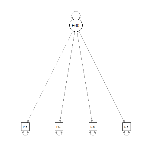
library(semPlot)
semPaths(fit)

Now we have a basic digram of our model. The dotted line from y1 to F60 indicates that this loading was fixed (in this case at 1). Rounded arrows pointing at each of the variables reflect their variance.
We could honestly stop here, but why? Let's have some fun with semPlot. First of all, we could give it a title. By adding line=3, I keep the title from appearing right on top of the latent variable (and covering up the variance).
semPaths(fit)
title("Political Democracy in 1960", line=3)

I could also add the parameter estimates to my figure. They default to large green text, so I prefer to change it to black (edge.color="black") and a smaller font size (edge.label.cex=0.75).
semPaths(fit, what="par", edge.label.cex=0.75, edge.color="black")
title("Political Democracy in 1960", line=3)

colnames(PoliticalDemocracy)<-c("Press.60","PolOp.60","Elect.60","Leg.60",
                                "Press.65","PolOp.65","Elect.65","Leg.65",
                                "GNP.60","Energy.60","Labor.60")
Free.Model <- 'Fr60 =~ Press.60 + PolOp.60 + Elect.60 + Leg.60'
fit <- sem(Free.Model, data=PoliticalDemocracy)
semPaths(fit, what="std",nCharNodes=0, edge.label.cex=1, sizeMan=10, edge.color="black")
title("Political Democracy in 1960", line=3)

Other fun tricks:
There are three different layout options: tree (default), circle, and spring. Here's what the other two look like.
semPaths(fit, layout="circle")

semPaths(fit, layout="spring")

semPaths(fit, rotation=1) #This is also the default
semPaths(fit, rotation=2)

semPaths(fit, rotation=3)

semPaths(fit, rotation=4)

We can change the appearance of errors. "mx" is the default, but another option is "lisrel".
semPaths(fit, style="lisrel")

And final trick I'll show: we can add some descriptive text to our model drawing.
semPaths(fit,rotation=2)
text(-0.5,-1.0,labels="Using the Bollen 1989\n Industrialization Political Democracy dataset\navailable in the lavaan package")

No comments:
Post a Comment