Statistics Sunday: Creating a Stacked Bar Chart for Rank Data

At work on Friday, I was trying to figure out the best way to display some rank data. What I had were rankings from 1-5 for 10 factors considered most important in a job (such as Salary, Insurance Benefits, and the Opportunity to Learn), meaning each respondent chose and ranked the top 5 from those 10, and the remaining 5 were unranked by that respondent. Without even thinking about the missing data issue, I computed a mean rank and called it a day. (Yes, I know that ranks are ordinal and means are for continuous data, but my goal was simply to differentiate importance of the factors and a mean seemed the best way to do it.) Of course, then we noticed one of the factors had a pretty high average rank, even though few people ranked it in the top 5. Oops.

So how could I present these results? One idea I had was a stacked bar chart, and it took a bit of data wrangling to do it. That is, the rankings were all in separate variables, but I want them all on the same chart. Basically, I needed to create a dataset with:

1 variable to represent the factor being ranked
• 1 variable to represent the ranking given (1-5, or 6 that I called "Not Ranked")
• 1 variable to represent the number of people giving that particular rank that particular factor

What I ultimately did was run frequencies for the factor variables, turn those frequency tables into data frames, and merged them together with rbind. I then created chart with ggplot. Here's some code for a simplified example, which only uses 6 factors and asks people to rank the top 3.

First, let's read in our sample dataset - note that these data were generated only for this example and are not real data:

library(tidyverse)

## -- Attaching packages --------------------------------------------------------------------------------------------------------------------- tidyverse 1.2.1 --

## v ggplot2 3.0.0     v purrr   0.2.4
## v tibble  1.4.2     v dplyr   0.7.4
## v tidyr   0.8.0     v stringr 1.3.1
## v readr   1.1.1     v forcats 0.3.0

## Warning: package 'ggplot2' was built under R version 3.5.1

## -- Conflicts ------------------------------------------------------------------------------------------------------------------------ tidyverse_conflicts() --
## x dplyr::filter() masks stats::filter()
## x dplyr::lag()    masks stats::lag()

ranks <- read_csv("C:/Users/slocatelli/Desktop/sample_ranks.csv", col_names = TRUE)

## Parsed with column specification:
## cols(
##   RespID = col_integer(),
##   Salary = col_integer(),
##   Recognition = col_integer(),
##   PTO = col_integer(),
##   Insurance = col_integer(),
##   FlexibleHours = col_integer(),
##   OptoLearn = col_integer()
## )

This dataset contains 7 variables - 1 respondent ID and 6 variables with ranks on factors considered important in a job: salary, recognition from employer, paid time off, insurance benefits, flexible scheduling, and opportunity to learn. I want to run frequencies for these variables, and turn those frequency tables into a data frame I can use in ggplot2. I'm sure there are much cleaner ways to do this (and please share in the comments!), but here's one not so pretty way:

salary <- as.data.frame(table(ranks$Salary))
salary$Name <- "Salary"
recognition <- as.data.frame(table(ranks$Recognition))
recognition$Name <- "Recognition by \nEmployer"
PTO <- as.data.frame(table(ranks$PTO))
PTO$Name <- "Paid Time Off"
insurance <- as.data.frame(table(ranks$Insurance))
insurance$Name <- "Insurance"
flexible <- as.data.frame(table(ranks$FlexibleHours))
flexible$Name <- "Flexible Schedule"
learn <- as.data.frame(table(ranks$OptoLearn))
learn$Name <- "Opportunity to \nLearn"

rank_chart <- rbind(salary, recognition, PTO, insurance, flexible, learn)
rank_chart$Var1 <- as.numeric(rank_chart$Var1)

With my not-so-pretty data wrangling, the chart itself is actually pretty easy:

ggplot(rank_chart, aes(fill = Var1, y = Freq, x = Name)) +
  geom_bar(stat = "identity") +
  labs(title = "Ranking of Factors Most Important in a Job") +
  ylab("Frequency") +
  xlab("Job Factors") +
  scale_fill_continuous(name = "Ranking",
                      breaks = c(1:4),
                      labels = c("1","2","3","Not Ranked")) +
  theme_bw() +
  theme(plot.title=element_text(hjust=0.5))

Based on this chart, we can see the top factor is Salary. Insurance is slightly more important than paid time off, but these are definitely the top 2 and 3 factors. Recognition wasn't ranked by most people, but those who did considered it their #2 factor; ditto for flexible scheduling at #3. Opportunity to learn didn't make the top 3 for most respondents.

Natural Graph

Via Not Awful and Boring, this reddit post discusses a really cool natural graph, measuring the amount of sunlight per day, created with a tree and a magnifying glass:

Apparently, this device is a Campbell-Stokes recorder.

Long Time, No Write

Wow, it's been way too long since I've posted anything! Lots of life changes recently, including moving to a new place and fighting with Comcast to get internet there. I still need to set up my office, and I plan on doing lots of writing in my new dedicated space. I'm planning on more statistics posts and a few more surprises this year.

Work has also been busy. At the moment:

• I'm working on three content validation studies, including analyzing data for two job analysis surveys and gearing up for a third
• I've wrapped up the first phase of analysis on our salary and satisfaction survey, and have some cool analysis planned for phase 2
• I finished a time study on our national and state exams
• I'm awaiting feedback on the first draft of a chapter about standard setting I coauthored with some coworkers
• I'm learning how to be a supervisor, now that I have someone working for me! That's right, I'm no longer a department of one

Once I get through some of the most pressing project work, I'm going to take some of my work time to teach myself data forensics as it applies to the testing. In fact, this book has been on my to-read shelf since my annual employee evaluation back in November. Look for blog posts on that!

Amazing Demonstration of the Digits of Pi

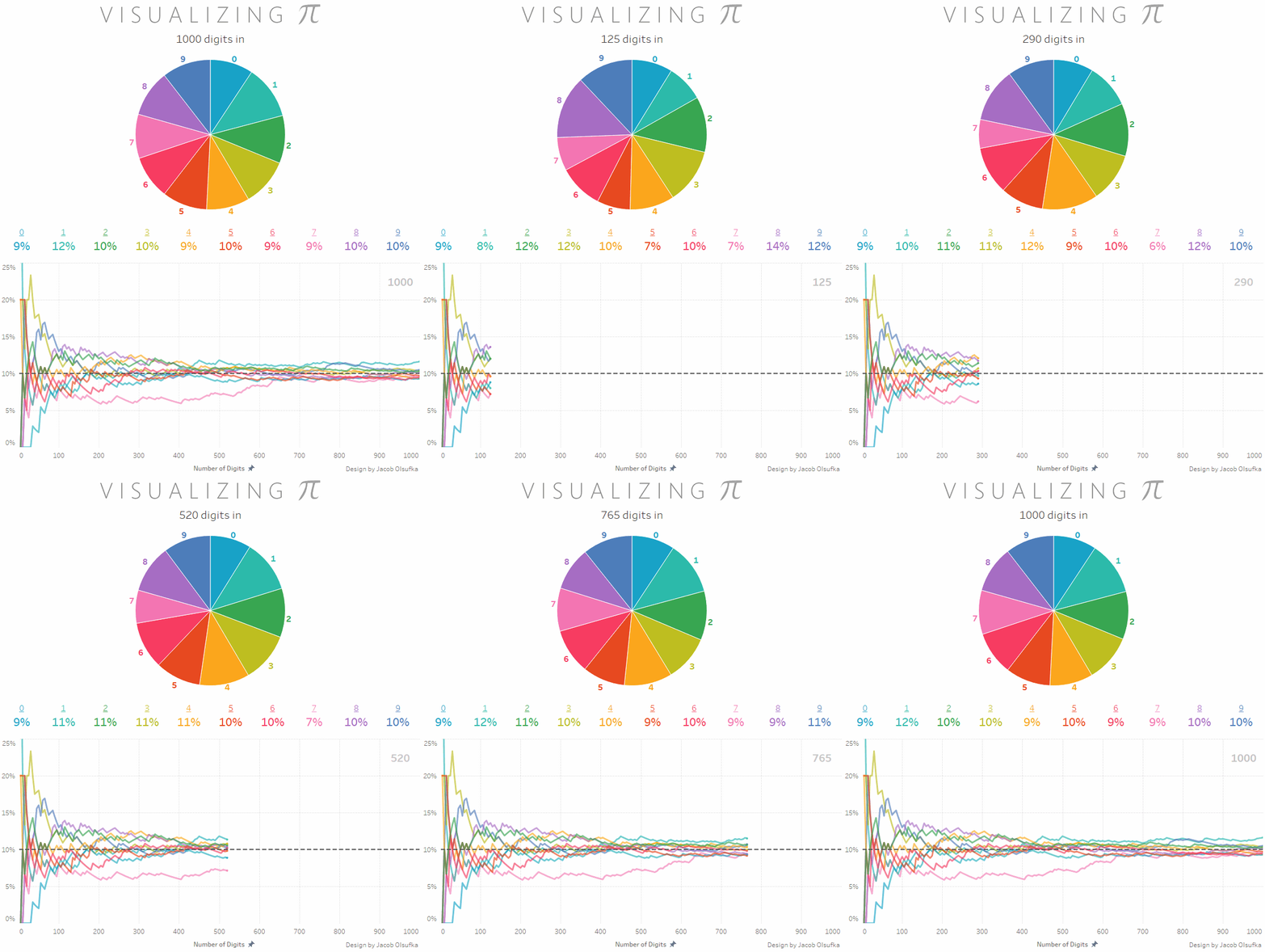
You probably know that pi made up of a series of digits that theoretically go on forever. Scientists have computers calculating the digits of pi, making it up to 2 quadrillion! Today, I found this great GIF that shows the count of digits (0 through 9) in the first 1000 digits of pi - pretty cool:

Statistics Sunday: Introduction to Regular Expressions

In my last Statistics Sunday post, I briefly mentioned the concept of regular expressions, also known as regex (though note that in some contexts, these refer to different things - see here). A regular expression is a text string, which you ask your program to match. You can use this to look for files with a particular name or extension, or search a corpus of text for a specific word or word(s) that match a certain pattern. This concept is used in many programming languages, and R is no exception. In order to use a regular expression, you need a regular expression engine. Fortunately, R base and many R packages come with a regular expression engine, which you call up with a function. In R base, those functions are things like grep, grepl, regexpr, and so on.

Today, I want to talk about some of the syntax you use to describe different patterns of text characters, which can include letters, digits, white space, and punctuation, starting from the most simple regular expressions. Typing out a specific text string matches only that. In last week's example, I was working with files that all start with the word "exam." So if I had other files in that folder that didn't follow that naming convention, I could look specifically for those by simply typing exam into the pattern attribute of my list.files() function. These files follow exam with a date, formatted as YYYYMMDD, and a letter to delineate each file from that day (a to z). Pretty much all of our files end in a, but in the rare instances where they send two files for a day, that one would end in b. How can I write a regular expression that matches this pattern?

First, the laziest approach, using the * character (which is sometimes called a greedy operator), which tells the regular expression engine to look for any number of characters following a string. For that, I could use this pattern:

list.files(pattern = "exam*")

A less lazy approach that still uses the + greedy operator would be specify the numbers I know will be the same for all files, which would be the year, 2018. In fact, if all of my exam files from every year were in a single folder, I could use that to select just one year:

list.files(pattern = "exam2018*")

Let's say I want all files from October 2018. I could do this:

list.files(pattern = "exam201810*")

That might be as fancy as I need to get for my approach.

We can get more specific by putting information into brackets, such as [a-z] to tell the program to match something with a lowercase letter in that range or [aA] to tell the program to look for something with either lowercase or uppercase a. For example, what if I wanted to find every instance of the word "witch" in The Wizard of Oz? Sometimes, the characters refer to a specific witch (Good Witch, Bad Witch, and so on) or to the concept of being a witch (usually lowercase, such as "I am a good witch"). I could download The Wizard of Oz through Project Gutenberg (see this post for how to use the guternbergr package; the ID for The Wizard of Oz is 55), then run some text analysis to look for any instance of Witch or witch:

witch <- WoO[grep("[Ww]itch", WoO$text),]

Here's what the beginning of the witch dataset looks like:

> witch
# A tibble: 141 x 2
   gutenberg_id text     
         <int> <chr>                                                                   
1           55 "  12.  The Search for the Wicked Witch"                                 
2           55 "  23.  Glinda The Good Witch Grants Dorothy's Wish"                     
3           55 We are so grateful to you for having killed the Wicked Witch of the     
4           55 killed the Wicked Witch of the East?  Dorothy was an innocent, harmless 
5           55 "\"She was the Wicked Witch of the East, as I said,\" answered the little"
6           55 " where the Wicked Witch ruled.\""   
7           55 When they saw the Witch of the East was dead the Munchkins sent a swift   
 8           55 "messenger to me, and I came at once.  I am the Witch of the North.\""   
 9           55 "\"Oh, gracious!\" cried Dorothy.  \"Are you a real witch?\""             
10           55 "\"Yes, indeed,\" answered the little woman.  \"But I am a good witch, and"
# ... with 131 more rows

I'm working on putting together a more detailed post (or posts) about regular expressions, including more complex examples and the components of a regular expression, so check back for that soon!

Statistics Sunday: Reading and Creating a Data Frame with Multiple Text Files

First Statistics Sunday in far too long! It's going to be a short one, but it describes a great trick I learned recently while completing a time study for our exams at work.

To give a bit of background, this time study involves analzying time examinees spent on their exam and whether they were able to complete all items. We've done time studies in the past to select time allowed for each exam, but we revisit on a cycle to make certain the time allowed is still ample. All of our exams are computer-administered, and we receive daily downloads from our exam provider with data on all exams administered that day.

What that means is, to study a year's worth of exam data, I need to read in and analyze 365(ish - test centers are generally closed for holidays) text files. Fortunately, I found code that would read all files in a particular folder and bind them into a single data frame. First, I'll set the working directory to the location of those files, and create a list of all files in that directory:

setwd("Q:/ExamData/2018")
filelist <- list.files()

For the next part, I'll need the data.table library, which you'll want to install if you don't already have it:

library(data.table)
Exams2018 <- rbindlist(sapply(filelist, fread, simplify = FALSE), use.names = TRUE, idcol = "FileName")

Now I have a data frame with all exam data from 2018, and an additional column that identifies which file a particular case came from.

What if your working directory has more files than you want to read? You can still use this code, with some updates. For instance, if you want only the text files from the working directory, you could add a regular expression to the list.files() code to only look for files with ".txt" extension:

list.files(pattern = "\\.txt$")

If you're only working with a handful of files, you can also manually create the list to be used in the rbindlist function. Like this:

filelist <- c("file1.txt", "file2.txt", "file3.txt")

That's all for now! Hope everyone has a Happy Thanksgiving!

Great Post on Using Small Sample Sizes to Make Decisions

It's been a busy month with little time for blogging, but I'm planning to get back on track soon. For now, here's a great post on the benefits of using small samples to inform decisions:

When it comes to statistics, there are a lot of misconceptions floating around. Even people who have scientific backgrounds subscribe to some of these common misconceptions. One misconception that affects measurement in virtually every field is the perceived need for a large sample size before you can get useful information from a measurement.

[I]f you can learn something useful using the limited data you have, you’re one step closer to measuring anything you need to measure — and thus making better decisions. In fact, it is in those very situations where you have a lot of uncertainty, that a few samples can reduce uncertainty the most. In other words, if you know almost nothing, almost anything will tell you something.

The article describes two approaches - the rule of five (taking a random sample of 5 to draw conclusions) or the urn of mystery (that a single case from a population can tell you more about the makeup of that population). The rule of five seems best when trying to get a continuous value (such as, in the example from the post, the average commute time of workers in a company), while the urn of mystery seems best when trying to determine if a population is predominantly one of two types (in the post, the example is whether an urn of marbles contains predominantly marbles of a certain color).

Obviously, there are times when you need more data. But if you're far better off making decisions with data (even very little) than with none at all.